Friday, 10 November 2023

Mathematical Definition of Heuristic Causal Inference:
What differentiates DAGs and do-calculus?

Preamble 

David Hume
David Hume (Wikipedia)
Experimental design is not a new concept and randomised control trials (RCTs) are our solid gold standard of doing quantitative research, when no apparent physical laws are available to validate observations.  However, it is very expensive to design RCTs, not ethical or either not possible due to logistical reasons in some cases. Then we fall into Causal Inference's heuristic frameworks, such as potential outcomes, matching, and time-series interventions in imagining counterfactuals and interventions. These methods provide immensely successful toolbox for quantitative scientist where by systems do not have any known physical laws. DAGs and do-calculus, differentiates from all these approaches that try to move away from full heuristics. In this post we try to postulate this formally in mathematical terms in the context of causal inference over observational data framework. We established that DAGs and do-calculus bring  mathematically more principled way of practicing causal inference akin to theoretical physics attitude. 

Definition of Heuristic Causal Inference (HeuristicCI) : Observational Data 

Heuristics in general implies an algorithmic approximate solution, usually appear as numerical and statistical algorithms in causal inference whereby full RCT is not available. This can be formalised as follows, 

Definition (HeuristicCI) Given dataset of  $n-$dimensions $\mathscr{D} \in \mathbb{R}^{n}$ observation, having variates of $X=x_{i}$, with each having different sub-sets (categories within $x_{i}$), having at least one category of observations.  We want to test  causal connection between two distinct subsets of $X$,  $\mathscr{S}_{1} , \mathscr{S}_{2}$, given an interventional versions or imagined counterfactual where by at least one of the subset is available,  $\mathscr{S}_{1}^{int} , \mathscr{S}_{2}^{int}$. Using an algorithm $\mathscr{A}$ that processes dataset to test an effect size $\delta$ using a statistic $\beta$,  as follows, $$ \delta= \beta(\mathscr{S}_{1} , \mathscr{S}_{1}^{int})-\beta(\mathscr{S}_{2} , \mathscr{S}_{2}^{int})$$ statistic $\beta$ can be result of a machine learning procedure as well and difference in $\delta$ is only a particular choice, i.e., such as Average Treatment Effect (ATE). The algorithm  $\mathscr{A}$ is called  HeuristicCI.

Many of the non-DAGs and do-calculus methods directly falls into this category, such as potential outcomes, upliftmatching and synthetic controls.  This definition could be quite obvious to practitioners that has a good handle in mathematical definitions. Moreover, HeuristicCI  implies solely data-driven approach to causality inline with Hume's pure-empirical view-point. 

Primary distinction in practicing DAGs that it brings causal ordering naturally [suezen23pco] with scientist's cognitive process encoded, where by HeuristicCI search for statistical effect size that has a causal component in fully data-driven way. However, a HybridCI would entails using DAGs and do-calculus in connection with data driven approaches.

Conclusion

In this short exposition, we introduced HeuristicCI  concept that category of methods that do not use DAGs and do-calculus explicitly in causal inference practice. However, we do not put a well designed RCTs  in this category. Because, as a gold standard approach whereby properly encoded experimental design generates full interventional data reflecting scientist's domain knowledge. 

References and Further reading

Please cite as follows:

 @misc{suezen23hci, 
     title = {Mathematical Definition of Heuristic Causal Inference: What differantiates DAGs and do-calculus?}, 
     howpublished = {\url{https://science-memo.blogspot.com/2023/11/heuristic-causal-inference.html}, 
     author = {Mehmet Süzen},
     year = {2023}
}  

Postscript A: Why Pearlian Causal Inference is very significant progress for empirical science? 

Judea Pearl's framework for causality sometimes referred to as “mathematisation of causality”. However, “axiomatic foundations of causal inference” is fair identification, Pearl's contribution to the field is in par with Kolmogorov's axiomatic foundations of probability. Key papers of this axiomatic foundations are published in 1993 (back-doors) [1] and 1995 (do-calculus) [2].  


Original works of Axiomatic foundation for causal inference:

[1] Pearl, J., “Graphical models, causality, and intervention,” Statistical Science, Vol. 8, pp. 266–269, 1993. 

[2] Pearl, J., “Causal diagrams for empirical research,” Biometrika, Vol. 82, Num. 4, pp. 669–710, 1995. 

Saturday, 1 April 2023

Resolution of misconception of overfitting: Differentiating learning curves from Occam curves

Preamble 

Occam (Wikipedia)
A misconception that overfitted model can be identified with the  amount of generalisation gap between model's training and test sets over its learning curves is still out there. Even in some prominent online lectures and blog posts, this misconception is now repeated without critical look. In general, this practice unfortunately diffuse into some academic papers and industrial,  practitioners attribute poor generalisation to overfitting. We have provided a resolution of this via a new conceptual identification of complexity plots, so called Occam's curves differentiating from a learning curve. An accessible mathematical definitions here will clarify the resolution of the confusion.   

Learning Curve Setting: Generalisation Gap 

Learning curves explain how a given algorithm's generalisation improves over time or experience, originating from Ebbinghaus's work on human memory.  We use inductive bias to express a model, as model can manifest itself in different forms from differential equations to deep learning.

Definition: Given inductive bias $\mathscr{M}$ formed by $n$ datasets with monotonically increasing sizes  $\mathbb{T} = \{|\mathbb{T}_{0}| > |\mathbb{T}_{1}| > ...> |\mathbb{T}_{n}| \}$. A learning curve $\mathscr{L}$ for $\mathscr{M}$ is expressed by the performance measure of the model over datasets,  $\mathbb{p} = \{ p_{0},  p_{1}, ... p_{n} \}$, hence $\mathscr{L}$ is a curve on the plane of $(\mathbb{T}, p)$.  

By this definition, we deduce that $\mathscr{M}$ learns if $\mathscr{L}$ increases monotonically. 

A generalisation gap is defined as follows. 

Definition: Generalisation gap for inductive bias $\mathscr{M}$ is the difference between its' learning curve $\mathscr{L}$ and the learning curve of the unseen datasets, i.e., so-called training, $\mathscr{L}^{train}$. The difference can be simple difference, or a measure differentiating the gap.

We conjecture the following. 

Conjecture: Generalisation gap can't identify if $\mathscr{M}$ is an overfitted model. Overfitting is about Occam's razor, and requires a pairwise comparison between two inductive biases of different complexities.

As conjecture suggests that generalisation gap is not about overfitting, despite the common misconception. Then, why the misconception? The misconception lies on the confusion of how to produce the curve that we could judge overfitting. 

Occam Curves: Overfitting Gap [Occam's Gap] 

In the case of generating Occam curves, a complexity measure  $\mathscr{C}$  over different inductive biases $\mathscr{M_{i}}$ plays a role. Then the definition reads. 

Definition: Given $m$ inductive bias $\mathscr{M_{i}}$ formed by $n$ datasets with monotonically increasing sizes  $\mathbb{T} = \{|\mathbb{T}_{0}| > |\mathbb{T}_{1}| > ...> |\mathbb{T}_{n}| \}$. An Occam curve $\mathscr{O}$ for a given $\mathscr{M}$ is expressed by the performance measure of the model over complexity-dataset size points  $\mathbb{F} = [(|\mathbb{T}_{0}|, \mathscr{C}),  (|\mathbb{T}_{1}| , \mathscr{C}), ...,  (|\mathbb{T}_{n}| , \mathscr{C}) ] $; Performance of a given inductive bias reads $\mathbb{p} = \{ p_{0},  p_{1}, ... p_{n} \}$, hence Occam curve, $\mathscr{O}$ is a curve on the plane of $(\mathbb{F}, p)$.  
 
Given definition, producing Occam curves are more complicated than simply plotting test and train curves over batches. The ordering in $\mathbb{F}$ forms what is so-called goodness of rank.

Summary and take home

Resolution of misconception of overfitting lies in producing Occam curves to judge the bias-variance tradeoff, not the learning curves of a single model. 

Further reading & notes

  • Further posts and a glossary : The concept of overgeneralisation and goodness of rank.
  • Double decent phenomenon, it uses Occam's curves, not learning curves.
  • We use dataset size as an interpretation of increasing experience, there could be other ways of expressing a gained experience, but we take the most obvious evidence.
Please cite as follows:

 @misc{suezen23rmo, 
     title = {Resolution of misconception of overfitting: Differentiating learning curves from Occam curves}, 
     author = {Mehmet Süzen},
     year = {2023}
}  

Postscript notes

Take home messages

Understanding Generalisation Gap and Occam’s gap

Model selection and evaluations are usually confused by novice and as well as experienced data scientists and professionals doing modelling. There are a lot of misconceptions in the literature, but in practice primary take home messages can be summarised as follows:

1. What is a model? A model is an “inductive bias” of the modeller, a selected parametrised functions for example, a neural network architecture choice. Contrary to many, specific parametrisation of a model (deep learning architecture) is not a different model.
2. A model’s test and training performance difference is about generalisation gap. Overfitting and under-fitting is not about generalisation gap.
3. Overfitting or under-fitting is a comparison problem: How a model deviates from a reference model? This is called Occam’s gap or so called model selection error.
4. Occam’s gap generalises Empirical Risk minimisation over a learning curve.  Empirical risk minimisation itself is not about learning.

How and when a model generalises well and generalisation of empirical risk minimisation are currently an open research topics.

Saturday, 25 February 2023

Loschimidt's Paradox and Causality:
Can we establish Pearlian expression for Boltzmann's H-theorem?

Boltzmann (Wikipedia)

Preamble

Probably the most important achievement for humans is the ability to produce scientific discoveries, that  helps us objectively understand how nature works and build artificial tools where no other species can.  Entropy is an elusive concept and one of the crown achievements of human race. We question here if causal inference and Loschmidt's paradox can be reconciled. 


Mimicking analogies are not physical

Before even try to understand what is a physical entropy, we should make sure that there is only one kind of physical entropy from thermodynamics, formulated by Gibbs-Boltzmann ($S_{G}$ and $S_{B}$).  Other entropies such as Shannon's information entropy are all analogies to physics, and mimicking concepts.

Why counting microstates are associated with time?

The following definition of entropy is due to Boltzmann but Gibbs' formulation tend to provide equivalence, technically different formulations aside, they are actually equivalent.

Definition 1: An entropy of a macroscopic material is associated with larger number of states its constituted elements take different states, $\Omega$. This is associated with $S_{B}$, Boltzmann's entropy.  

Now, as we know from basic thermodynamics classes that entropy change of a system can not decrease, so the time's arrow. 

Definition 2: Time's arrow is identified with change in entropy of material systems, that $\delta S \ge 0$.

We put aside the distinction between open and close systems and equilibrium and non-equilibrium dynamics, but concentrate on how come counting system's state's are associated with time's arrow? 

Loschimidt's Paradox: Irreversible occupancy on discrete states and causal inference

The core idea probably can be explained via discrete lattice and occupancy on them over chain of dynamics. 

Conjecture 1: Occupancy of $N$ items on $M$ discrete states, $M>N$, evolving with dynamical rules $\mathscr{D}$ necessarily increases $\Omega$, compare to the number of sampling if it were $M=N$. 

This conjecture might explain the entropy increase, but irreversibility of the dynamical rule $\mathscr{D}$ is required addressing Loschimidt's Paradox, i.e., how to generate irreversible evolution given time-reversal dynamics. Actually, do-calculus may provide a language to resolve this, by inducing interventional notation on Boltzmann's H-theorem with Pearlian view. The full definition of H-function is a bit more involved, but here we summarise it in condensed form with a do operator version of it.

Conjecture 2 (H-Theorem do-conjecture): Boltzmann's H-function provides a basis for entropy increase, it is associated with conditional probability of a system $\mathscr{S}$ being in state $X$ on ensemble $\mathscr{E}$. Hence, $P(X|\mathscr{E})$. Then, an irreversible evolution from time-reversal dynamics should use interventional notation, $P(X|do(\mathscr{E}))$. Then information on how time reversal dynamics leads to time's arrow encoded on, how dynamics provides an interventional ensembles, $do(\mathscr{E})$.

Conclusion

We provided some hints on why would counting states lead to time's arrow, an irreversible dynamics.  In the light of the development of mathematical language for causal inference in statistics, the concepts are converging. Along with understanding Loschmidt's Paradox via do-calculus, it can establish an asymmetric notation. Loschmidt's question is long standing problem in physics and philosophy with great practical implications in different physical sciences.

Further reading

Please cite as follows:

 @misc{suezen23lpc, 
     title = {Loschimidt's Paradox and Causality: Can we establish Pearlian expression for Bolztmann's H-theorem?}, 
     howpublished = {\url{https://science-memo.blogspot.com/2023/02/loschimidts-do-calculus.html}}, 
     author = {Mehmet Süzen},
     year = {2023}
}  

@article{suzen23htd,
    title={H-theorem do-conjecture},
    author={Mehmet Süzen},
    preprint={arXiv:2310.01458},
    url = {https://arxiv.org/abs/2310.01458}
    year={2023}
}

Saturday, 18 February 2023

Insights into Bekenstein entropy with an intuitive mathematical definitions:
A look into Thermodynamics of Black-holes

Jacob Bekenstein
(Wikipedia)
Preamble

Thermodynamics of black holes has appeared as one of the most interesting areas of research in theoretical physics [Wald1994], specially after LIGO's massive success. The striking results of Jacob Bekenstein  [Bekenstein1973] in proposing a formulation of entropy for a black hole was on of the most striking turning point in building explanations for the thermodynamics of gravitational systems. Bekenstein entropy is defined to be so-called a phenomenological relationship and surprisingly easy to understand concept using basic dimensionality analysis. In this post, we will show how to understand the entropy of a black hole just using basic dimensionality analysis, fundamental physics constants and basic definition of entropy. 

Dimensions and scales

Dimensionality analysis appears in many different areas of physics and engineering, from fluid dynamics to relativity. The starting point is to understand the concept of dimensions. Every quantity we measure in real life has a dimension. It means a quantity $\mathscr{Q}$  we obtain from a measurement $\mathscr{M}$ has a numeric value $v$ and associated unit $u$. $\mathscr{Q}=\langle  v, u \rangle$ given $\mathscr{M}$. There are 3 distinct fundamental unit types length (L),  time (T) and mass (M).

Intuitive Bekenstein entropy (BE) for a black hole : Informal mathematical definition

Black holes are astronomical objects that are not directly observable due to their mass condensed in a small area. The primary object we will use is something called Planck length $L_{p}$ and it implies physically possible smallest patch of the space-time, this is associated with the state of the black holes on their horizon. We won't define the Planck length here in detail but with the knowledge of fundamental physics constants and dimensional analysis we mentioned, one can get a constant value for this length. 

Definition: Finite entropy $S_{f}$ of an object is associated with the number of states $\Omega$ a system can attain.

If we combine this definition for a black hole entropy : 

Definition Finite entropy of a black-hole $S_{f}^{BH}$ is  associated with the number of its states $\Omega$, number of elements on it's surface area of $A$. The elements are discretised with  small patches $a_{p}=L_{p}^{2}$. Then intuitively,  $\Omega$ yields to $A$ divided by $a_{p}$.
  
Bekenstein entropy is not thermodynamic entropy alone and family of Bekenstein entropies

The unit analysis tells us that $A$ has a dimension of length square.  We intentionally omit any equality in the above definition upon $S_{f}^{BH}$ because, in practice Bekenstein Entropy is not thermodynamic entropy alone. The formulation usually presented as BE in general uses equality for the above approach. However this is not strictly thermodynamical alone, that's why we specify definitions as finite entropy and only express the relationship as association. Similarly any other constants as it can yield to different Bekenstein entropies such as introduction of new constants would yield to family of Bekenstein entropies.

Why surface area defines states of a black-hole?

This is an amazing question and Bekenstein's main contribution is to associate this to number of states of a black-hole on event horizon, i.e., point of of no return layer whereby ordinary matter can't return. The justification is that all other properties of black hole defines this surface. Here is the intuitive definition of states of black-hole.

Definition A surface area $\mathscr{A}$ is formed by the set of physical properties forming an ensembles. such as charge density, angular momentum. These ensembles indirectly samples thermodynamics ensembles. 

Even though intuition is there, this question might still be an open question further.

Conclusion

We provided the primary idea that Bekenstein tried to convey in his 1973 paper intuitively. However,  we identify its thermodynamic limit is an open research area. Thermodynamic limit implies that taking infinite limit of both area and the discretised areas, even though it sounds that the values might converge to infinity, simultaneous limit would converge to a finite value for a physical matter. 

Primary Papers
Primary Book

Please cite as follows:

 @misc{suezen23ibe, 
     title = {Insights into Bekenstein entropy with an intuitive mathematical definitions}, 
     howpublished = {\url{https://science-memo.blogspot.com/2023/02/bekenstein-entropy.html}, 
     author = {Mehmet Süzen},
     year = {2023}
  }

Postscript A: 

Information can’t be destroyed


Proposals of that information is destroyed out of thin air is a red flag for any physical theory: this includes theories on evaporating black holes. Bekenstein’s insight in this direction that surface area is associated with entropy. The black-holes’   information in this context is quite different than the Shannon’s entropy. An evaporating black-hole, the area approaching to zero is not the same as information going to zero, surface area is a function of  physical properties of the stellar object that bound  by conservation laws in their interaction with their surrounding. Hence, the information is preserved even if area goes  to zero.


Postscript B: 

What is Holographic principle? its origins from Bekenstein Entropy perspective

The word embedding applies in this context as well. Embedding implies some sort of  dimensionality projection. A projection to lower dimensional space, or on the other end,  to the higher dimensional space. Holography is no different. Imagine taking 2D snap shots of rotating 3D objects, generating this in reverse is the end effect of holographic  reconstruction. N-dimension to (N-1) projection. This is the bases of holographic principle: entropy of black-holes doesn’t appear as all states of its constituted matter,  as normally should have for ordinary matter, it manifest as N-1 projection on it’s surface. This kind of holographic entropy is first noted by Bekenstein; whereby he assigned the event-horizon area as a representation of the states of the black-hole volume. This projection to (N-1)-dimension is improved upon Bekenstein’s approach to generalised situations in explaining how universe might be  a hologram entirely by Gerard 't Hooft and Leonard Susskind. Holographic principle, probably one of the most important development in theoretical physics in recent times.


Saturday, 28 January 2023

Misconceptions on non-temporal learning: When do machine learning models qualify as prediction systems?

Preamble

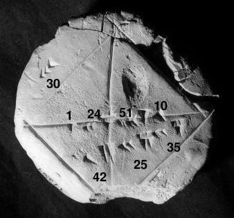
    Babylonian Tablet for 
square root of 2.
 (Wikipedia)
Prediction implies a mechanics, as in knowing a form of a trajectory over time.  Strictly speaking a predictive system implies knowing a solution to the path, set of variable depending on time, time evolution of the system under consideration. Here, we define semi-informally how a prediction system is defined mathematically and show how non-temporal learning can be mapped into a prediction system. 

Temporal learning : Recurrence, trajectory and sequences

A trajectory can be seen as a function of time, identified in recurrence manner. It means $x(t_{i})=f(x_{i-1})$. However, this is one of the possible definitions. The physical equivalent of this appears as a solution to ordinary differential equation, such as the velocity $v(t) = dx(t)/dt$, recurrence on its solution. On the other hand machine learning, an empirical approach is taken and a sequence data such as natural language or a log events occurring in sequence. Any modelling on such data is called temporal learning. This includes classical time-series algorithms, gated units in deep learning and differential equations.

Definition: A prediction system  $\mathscr{F}$ that is build with data $D$ but utilised for a data that is not used in building it $D'$, qualified as such if both $D$ and $D'$ are temporal sets and output of the system is a horizon $\mathbb{H}$, that is a sequence. 

Using non-temporal supervised learning is interpolation or extrapolation

Often practice in industry to turn temporal interactions into flat set of data vectors,  $v_{i}$, $i$ corresponds to a time point or an arbitrary property of the dataset resulting in breaking the temporal associations and causal links.  This could also manifest as set of images with some labels which has no ordering or associational property in the dataset. Even though our system build upon these non-temporal datasets, indeed it constituted a learning systems as interpolation or extrapolation. Their utility in using them for $D'$, strictly speaking does not qualify as prediction systems. 

Mapping with pre-processing

A mapping indeed possible from non-temporal data to a temporal one, if their original form is not in temporal form yet. This is been studied in complexity literature. This requires an algorithm to map flattened data vectors we mentioned into a sequence data. 

Mapping with Causality

A distinct models from causal inference are qualified as predictive systems even if they are trained on non-temporal data, because causality establishes a temporal learning.

Non-temporal modals: Do they still learn?

Even though, we exclude non-temporal model utilisation as non-predictive systems, they still classified as learned models. Because their outputs are generated by a learning procedure. 

Conclusion

Differentiation among temporal and non-temporal learning is provided in associational manner. This results into definition of a prediction system, that excludes non-temporal machine learning models: such as models for unlinked set of vectors, a set of numbers mapped from any data modality. 

Further reading & postscript notes


(c) Copyright 2008-2024 Mehmet Suzen (suzen at acm dot org)

Creative Commons License
This work is licensed under a Creative Commons Attribution 4.0 International License.