Particle approximation to probability density functions: Dirac delta function representation

In the previous post, I have briefly shown the idea of using dirac delta function for discrete data representation. In the second example there, a histogram locations for a given set of points are presented as spike trains, where as heights are somehow given in a second sum. This is hard to follow and visualise, of course if you are not that good in reading formulation with different indexes. Due to pedagocial reasons, an easier representation of arbitrary probability density function (PDF), $p(x)$, one would simply need to couple each discrete points with a corresponding weight.

Hence, a set  $\{x_{i}, \omega^{i}\}_{i=1}^{N}$ would be an estimation of PDF, $\hat{p}(x)$ . At this point we can invoke dirac delta function,

$ \hat{p}(x) = \sum_{i=1}^{N} \omega^{i} \delta(x-x_{i})$

Let's revisit the R code given there, this time let's draw uniform numbers between $[-2, 2]$ to get 100  $x_{i}$ values. Simply these numbers will indicate the locations on the x-axis, a spike train.  For simplicity, let's use Gausian distribution for target PDF, $ \mathcal{N}(0, 1)$.  Than, for weights we need to draw numbers using the spike locations. This approach is easier to understand compare to my previous double index notation.

R Example code

Above explained procedure is trivial to implement in R.

1 2 3 4 5 6 7 8 9 10

# Generate locations 100 x locations # out out 1000 points in [-2.0, 2.0] set.seed(42) # Domain where Dirac comb operates Xj = seq(-2,2,0.002) Xi = sample(Xj, 100) # Now generate weights from N(0,1) at those given locations Wi = dnorm(Xi) # Now visualise plot(Xi, Wi, type="h",xlim=c(-2.0,2.0),ylim=c(0,0.6),lwd=2,col="blue",ylab="p")

Conclusion

Above notation introduces second  abuse of notation while actually there must be a secondary regular grid that pics $x_{i}$ values using dirac delta in practice. Because, the argument of $\hat{p}(x)$, is in the discrete domain. So a little better notation that reflects the above code would be

$ \hat{p}(x_j) = \sum_{i=1}^{N} \omega^{i} \delta(x_{j}-x_{i})$

The set $x_j$ is simply defined in a certain domain, for example regularly. Hence I only recommend not to introduce dirac delta for explaining a particle approximation to PDFs for novice students in the class. It will only confuse them even more.

Figure: Spike trains with weights $\hat{p}(x) = \sum_{i=1}^{N} \omega^{i} \delta(x-x_{i})$

Demystify Dirac delta function for data representation on discrete space

Dirac delta function is an important tool in Fourier Analysis. It is used specially in electrodynamics and signal processing routinely.  A function over set of data points
is often shown with a delta function representation. A novice reader relying on integral properties of the delta function may found this notation quite confusing.  Probably, the notation itself is an example of  abuse of notation.

One dimensional function/distribution: Sum of delta functions

Let's define a one dimensional function, $f(x)$ as follows, $x \in \mathbb{R}$ and $a$ being constant:

$ f(x) = a \sum_{i=-n}^{n} \delta(x - x_{i})$

This representation is inspired from Dirac comb and used in spike trains.  Note that set of data points in one dimension $\{x_{i} \}$ will determine the graph of this function. Using the shifting property of delta function, the value of the function will be zero every where except on data points. The constant $a$ will simply be the height of the graph at the data point.

Figure: A spike train.

Numeric Example

Let's plot $f(x)$ for some specific values of the set $\{x_{i} \} = {-0.5, -0.2, -0.1, 0.2, 0.4}$ and $a=0.5$. Here is the R code for plotting this spike train. 

x_i = c(-0.5, -0.2, -0.1, 0.2, 0.4)
a   = c(0.5, 0.5, 0.5, 0.5, 0.5)
plot(x_i,a,type="h",xlim=c(-0.6,0.6),ylim=c(0,0.6),lwd=2,col="blue",ylab="p") 

Representing Histograms: One dimensional example

Particularly convenient representation of histograms can be developed similarly. Consider set of points $\{x_{i}\}_{i=1}^{n}$ where we would like to establish a histogram out of this set, let's say $h(x)$. If we set our histogram intervals as $\{x_{j}\}_{j=1}^{m}$. The histogram $h(x)$ then can be written as

$h(x_{j}) =  \sum_{i=1}^{n} \sum_{j=1}^{m} \delta(x_{j}- x_{i}^{min})$
where set $x_{i}^{min}$  represents the value from set $\{x_{j}\}_{j=1}^{m}$ that is closest to given $x_{i}$. Where as, second sum determines the height at a given point, i.e., frequency. This is just a confusing mathematical representation and practical implementation only counts the frequency of $x_{i}^{min}$ directly.


Conclusion

However it is quite trivial, the above usage of sum of delta functions appear in mathematical physics as well, not limited to statistics.

N-body wave function has no meaning but shut up and calculate: quantum bayesianism

During my graduate school years I was lucky to be assigned on reporting a technique used in computational quantum chemistry, namely resolution of identity.  It is a simple trick to approximate many integrals with a smaller one. I don't want to discuss about this trick but rather a peculiar idea, if not controversial,  I come up during preparation of that report (here). It is about the legitimacy of wave function in many electron, let's be brave and say N-body, physical systems. Argument is posed by Walter Kohn, Nobel Physicist, in his lecture (here) attributed to Van Vleck:

I begin with a provocative statement. In general the
many-electron wave function $\Psi(r_{1} , . . . ,r_{N} )$ for a system
of $N$ electrons is not a legitimate scientific concept, when
$N \ge N_{0}$ , where $N_{0} = 10^{3}$ .

I believe this argument has a profound implication in interpretation of quantum mechanics. However,  sadly, perception of quantum mechanics in many circles of scientific community is limited to Schrödinger equation and interpretations based on wave function. Specially the concept of wave function collapse. In my view these approaches does not make any sense for macroscopic systems such as, humans. Considering Kohn's statement. I can only see the relevance in quantum computing where really small physical systems are in consideration. (Also see my previous post, pointing out recent works in constructing quantum mechanics without wave function)

One prominent figure in recent times is distinguished Professor Mermin who popularised the short version of Copenhagen interpretation as : 'shut up and calculate' and developer of the ithaka interpretation . Very recently discusses about quantum Bayesianism (here). Again, using Kohn's statement we have to be careful not to extent this concept, again, to macroscopic systems like Humans' or even larger atomic systems, like measurement devices. So, replacing a quantum measurement device with a human observer is a mistake, if not a sin. Doesn't matter even if they have a fancy names like Bob or Alice. Because a measurement device big enough has no defined or meaningful wave function hence any kind of  "quantum probability",  i.e., no superposition to observed systems can be established. Probably, problem lies in the transition from microscopic to macroscopic system. There was a large effort in this direction (here).

What ever you believe and read about quantum mechanics. I can only suggest that your crap detectors must function fully all the time when you hear some one talk about quantum mechanics and its interpretation, including this post. I recommend you Neil Postman's article Bullshit and the Art of Crap-Detection.

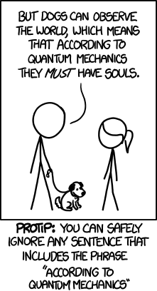
PS: Recently, there was an interesting cartoon on xkcd saying that we can safely ignore any phrase that starts with "According to quantum mechanics...".

Matrix Cumulative Coherence: Fourier Bases, Random and Sensing Matrices

Compressive sampling (CS) is revolutionizing the way we process analog to digital conversion, our understanding of linear systems and the limits of information theory. One of the key concept in CS is that a signal can be represented in a sparse bases or it is already sparse. The novelty of sparsity bases is that when signal is randomly sampled, in a nutshell it can be recovered (or a solution can be found to a linear problem) with fewer samples. A land mark example is being sparse MRI.

The concept of choosing "more" sparse bases or CS sensing matrix lies in the measure of mutual coherence. It is defined as follows for a given matrix at order k.
$$  M(A, k) = max_{p} max_{p \ne q, q \in \Omega } \sum_{q} | <a_{p}, a_{q}> | / ( |a_{p}| |a_{q}|)$$ When k=1, it is easy to understand what it means. Basically we find the largest inner product among columns of the given matrix. Lower the value better the sparsity i.e. incoherence. However a single number may not be so informative, after all how low is better.  With the definition of David Donoho and Joel Tropp,  if M is slowly increasing then matrix said to be enchances sparsity. Larger value of k forms a set of columns $\Omega$, and the second colums are selected from this set i.e. second max argument in the above definition.

In a recent post I have shortly reviewed my R package for CS called R1magic. Its recent version 0.2 contains a functionality to compute $M(A, k)$.  Also now there is a public Github repository of the package. mutualCoherence function is written fully functional way. All operations for computing $M(A,k)$ performed in vectorial fashion in R, using function closures and apply. However, for much larger matrices, a low level implementation may be required.

Example

Here we shortly investigate coherence of Fourier, random and mixed bases in R.

1 2 3 4 5 6 7 8 9 10 11 12 13 14 15 16

require("R1magic") set.seed(42) A <- DFTMatrix0(10) # Fourier Bases B <- matrix(rnorm(100), 10, 10) # Gaussian Random Matrix C <- A %*% B # A sensing matrix with A and B as above aa<-mutualCoherence(A, 8) bb<-mutualCoherence(A, 8) bb<-mutualCoherence(A, 8) aa [1] 1 1 1 1 1 1 1 1 bb [1] 0.6784574 1.2011489 1.7001046 2.1713561 2.4664608 2.7302690 2.7908302 [8] 2.9623327 cc [1] 0.7506222 1.3448452 1.8047043 2.1105348 2.3350516 2.4703822 2.5898766 [8] 2.6882250

We observe that mixed bases, where we define so called a CS matrix, matrix $C$ in above notation, with Fourier ($A$) and Random basis ($B$). Its mutual coherence increases slower than the pure random matrix with unit measure. This may signify a better incoherent basis.  However, since this is a "syntetic data', it does not tell any universal behaviour at all. A real data or signal measurement matrix  shall be tested for a better judgement of which bases is better to use in sparse recovery.  A recent paper in optical tomography uses this concept to identify a better sensing matrix in tomographic image reconstruction.