Basic understanding of a metric tensor: Disassemble the concept of a distance over Riemannian Manifolds

Preamble 

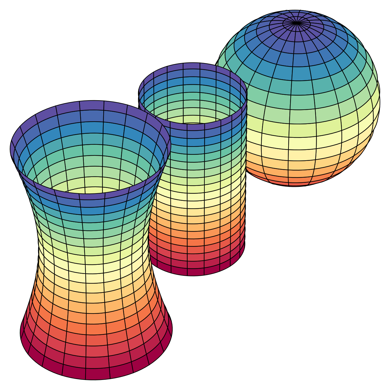
Gaussian Curvature (Wikipedia)

One of the core concepts in Physics is so called metric tensor. This object encodes any kind of geometry. Combined genius of Gauß,  Riemann and their contemporaries lead to such a great idea, probably one of the achievements of human quantitative enlightenment. However, due to notational aspects and lack of obvious pedagogical introduction, making object elusive mathematically. Einstein's notation made this more accessible but still, it requires more explicit explanation.  In this post we disassemble the definition of a distance over any geometry with an alternate notation. 

Disassemble distance over a Riemannian Manifolds

The most general definition of a distance between two infinitesimal points on any geometry, or a fancy word for it, is a Riemannian Manifolds, is defined with the following definitions. Manifold is actually a sub-set of any geometry we are concerned with and Riemannian implies a generalisation.

Definition 1: (Points on a Manifold) Any two points are defined in general coordinates $X$ and $Y$,  They are defined as row and column vectors respectively. In infinitesimal  components. $X = [dx_{1}, dx_{2}, ..., dx_{n}]$ and $Y= [dx_{1}, dx_{2}, ..., dx_{m}]^{T}$. 

Geometric description between two points are defined as tensor product, $\otimes$, that is to say we form a grid, on the geometry. 

Definition 2: (A infinitesimal grid) A grid on a geometry formed by pairing up each point's components, i.e., a tensor product. This would be a matrix $P^{mn}$, (as in points), with the first row $(dx_{1} dx_{1},.....,dx_{1} dx_{n})$ and the last row $(dx_{m} dx_{1},.....,dx_{m} dx_{n})$.

Note that grid here is used as a pedagogical tool, points are actually leaves on the continuous manifold. Now, we want to compute the distance between grid-points, $dS^{n}$, then metric tensor come to a rescue

Definition 3: (Metric tensor) A metric tensor $G^{nm}$ describes a geometry of the manifold that connects the infinitesimal grid to distance, such that $dS^{n}=G^{nm} P^{mn}$.

Note that, these definition can be extended to higher-dimensions, as in coordinates are not 1D anymore. We omit the square-root on the distance, as that''s also a specific to L2 distance.  Here, we can think of $dS^{n}$ a distance vector, and $G^{nm}$ and $P^{mn}$ are the matrices. 

Exercise: Euclidian Metric

A familiar geometry, metric for Euclidian space, reads diagonal elements of all 1 and rest of the elements zero. How the above definitions holds, left as an exercise. 

Conclusion 

We have discuss that a metric tensor, contrary to its name, it isn't a metric per se but an object that describes a geometry, having magic ability to connecting grids to distances. 

Further reading

There are a lot of excellent books out there but a classic Spivak's differential geometry is recommended. 

Please cite as follows:

 @misc{suezen24bumt, 

     title = {Basic understanding of a metric tensor: Disassemble the concept of a distance over Riemannian Manifolds}, 

     howpublished = {\url{https://science-memo.blogspot.com/2024/04/metric-tensor-basic.html}, 

     author = {Mehmet Süzen},

     year = {2024}

}  

Tensor Algebra: Efficient Operations on Multidimensional Arrays with R

 Multidimensional arrays are ubiquitous. Any complex problem having multivariate observables would easily generate a need to represent corresponding data in multidimensional arrays. Most of the practitioners would choose to apply operations on these objects with an index notation.  For example a 3-D array would have 3 indices A[i, j, k] or A[i][j][k] depending on the syntax. However there are languages which takes array operations as their native component, for example APL. More familiar examples are matrix operations in MATLAB, Fortran 90 and alike. Of course this concept is noting more than vectorisation.

Mathematical objects called tensors can be used to represent multidimensional objects. In reality a scalar is rank 0 tensor,  so scalar is the simplest tensor. Rank of a tensor can be thought as objects spatial dimension.  Let's consider matrix multiplication, where there are two indices, tensor of rank 2. If we have two matrices $A_{ij}$ and $B_{ij}$. We can multiply them with index notation as follows using an obscure language R with a naive algorithm:

> set.seed(42)
> A <- matrix(rnorm(4), 2, 2)
> B <- matrix(rnorm(4), 2, 2)
> C <- matrix(0, 2, 2)
> for(i in 1:2) {
+  for(j in 1:2) {
+   for(k in 1:2) {
+     C[i,j] = C[i,j] + A[i, k] * B[k,j]
+    }
+   }
+ }
> C
          [,1]       [,2]
[1,]  6.413566 -2.5178879
[2,] -2.249789  0.4908884
> A %*% B
           [,1]       [,2]
[1,]  0.5156982  2.0378605
[2,] -0.2954518 -0.9134599

You should have noticed that we introduce a third index. That is called a dummy index which we actually do the sum. This approach is technically called Einstein summation rule. So we represent the multiplication as follows: $C_{ij} = \sum_{k=1}^{m} A_{ik} B_{kj}$. Normally sum is dropped for short notation. It is quite intuitive from this notation that number of columns of A should be equal to number of rows in B to perform the sum consistently.

There are software packages that can do symbolic and numerical tensor algebra . Here we demonstrate an R package called tensorA developed by Professor van den Boogaart of TU Freiberg. We can repeat the matrix multiplication by using this package as follows.

> library("tensorA")
> set.seed(42)
> At <- to.tensor(rnorm(4), c(i=2, k=2))
> Bt <- to.tensor(rnorm(4), c(k=2, j=2))
> At %e% Bt
      j
i            [,1]       [,2]
  [1,]  0.5156982  2.0378605
  [2,] -0.2954518 -0.9134599
attr(,"class")
[1] "tensor" "matrix"

Note that here $\%e\%$ implies tensor multiplication with Einstein summation rule. This is pretty trivial example but if you imagine higher dimensional objects, tracking indices would be cumbersome so multi-linear algebra makes life easy.

In conclusion,  I think,  using tensor arithmetic for multidimensional arrays looks more compacts and efficient (~ 2-3 times).  A discussion related to this appeared in R help list.