Insights into Bekenstein entropy with an intuitive mathematical definitions: A look into Thermodynamics of Black-holes

Jacob Bekenstein
(Wikipedia)

Preamble

Thermodynamics of black holes has appeared as one of the most interesting areas of research in theoretical physics [Wald1994], specially after LIGO's massive success. The striking results of Jacob Bekenstein  [Bekenstein1973] in proposing a formulation of entropy for a black hole was on of the most striking turning point in building explanations for the thermodynamics of gravitational systems. Bekenstein entropy is defined to be so-called a phenomenological relationship and surprisingly easy to understand concept using basic dimensionality analysis. In this post, we will show how to understand the entropy of a black hole just using basic dimensionality analysis, fundamental physics constants and basic definition of entropy. 

Dimensions and scales

Dimensionality analysis appears in many different areas of physics and engineering, from fluid dynamics to relativity. The starting point is to understand the concept of dimensions. Every quantity we measure in real life has a dimension. It means a quantity $\mathscr{Q}$  we obtain from a measurement $\mathscr{M}$ has a numeric value $v$ and associated unit $u$. $\mathscr{Q}=\langle  v, u \rangle$ given $\mathscr{M}$. There are 3 distinct fundamental unit types length (L),  time (T) and mass (M).

Intuitive Bekenstein entropy (BE) for a black hole : Informal mathematical definition

Black holes are astronomical objects that are not directly observable due to their mass condensed in a small area. The primary object we will use is something called Planck length $L_{p}$ and it implies physically possible smallest patch of the space-time, this is associated with the state of the black holes on their horizon. We won't define the Planck length here in detail but with the knowledge of fundamental physics constants and dimensional analysis we mentioned, one can get a constant value for this length. 

Definition: Finite entropy $S_{f}$ of an object is associated with the number of states $\Omega$ a system can attain.

If we combine this definition for a black hole entropy : 

Definition Finite entropy of a black-hole $S_{f}^{BH}$ is  associated with the number of its states $\Omega$, number of elements on it's surface area of $A$. The elements are discretised with  small patches $a_{p}=L_{p}^{2}$. Then intuitively,  $\Omega$ yields to $A$ divided by $a_{p}$.

  

Bekenstein entropy is not thermodynamic entropy alone and family of Bekenstein entropies

The unit analysis tells us that $A$ has a dimension of length square.  We intentionally omit any equality in the above definition upon $S_{f}^{BH}$ because, in practice Bekenstein Entropy is not thermodynamic entropy alone. The formulation usually presented as BE in general uses equality for the above approach. However this is not strictly thermodynamical alone, that's why we specify definitions as finite entropy and only express the relationship as association. Similarly any other constants as it can yield to different Bekenstein entropies such as introduction of new constants would yield to family of Bekenstein entropies.

Why surface area defines states of a black-hole?

This is an amazing question and Bekenstein's main contribution is to associate this to number of states of a black-hole on event horizon, i.e., point of of no return layer whereby ordinary matter can't return. The justification is that all other properties of black hole defines this surface. Here is the intuitive definition of states of black-hole.

Definition A surface area $\mathscr{A}$ is formed by the set of physical properties forming an ensembles. such as charge density, angular momentum. These ensembles indirectly samples thermodynamics ensembles. 

Even though intuition is there, this question might still be an open question further.

Conclusion

We provided the primary idea that Bekenstein tried to convey in his 1973 paper intuitively. However,  we identify its thermodynamic limit is an open research area. Thermodynamic limit implies that taking infinite limit of both area and the discretised areas, even though it sounds that the values might converge to infinity, simultaneous limit would converge to a finite value for a physical matter. 

Primary Papers

• Bekenstein J.D.: Lettere al Nuovo Cimento, 4, 737, (1972)
• Bekenstein J.D.: Physical Review D, 7, 2333, (1973)  
• Bekenstein J.D.: Physical Review D, 9, 3292 (1974)
• Bekenstein J.D.: Physical Review D, 12, 3077 (1975)

Primary Book

• Wald, Quantum field theory in curved space times (1994) 

Please cite as follows:

 @misc{suezen23ibe, 

     title = {Insights into Bekenstein entropy with an intuitive mathematical definitions}, 

     howpublished = {\url{https://science-memo.blogspot.com/2023/02/bekenstein-entropy.html}, 

     author = {Mehmet Süzen},

     year = {2023}

  }

Postscript A: 

Information can’t be destroyed

Proposals of that information is destroyed out of thin air is a red flag for any physical theory: this includes theories on evaporating black holes. Bekenstein’s insight in this direction that surface area is associated with entropy. The black-holes’   information in this context is quite different than the Shannon’s entropy. An evaporating black-hole, the area approaching to zero is not the same as information going to zero, surface area is a function of  physical properties of the stellar object that bound  by conservation laws in their interaction with their surrounding. Hence, the information is preserved even if area goes  to zero.

Postscript B: 

What is Holographic principle? its origins from Bekenstein Entropy perspective

The word embedding applies in this context as well. Embedding implies some sort of  dimensionality projection. A projection to lower dimensional space, or on the other end,  to the higher dimensional space. Holography is no different. Imagine taking 2D snap shots of rotating 3D objects, generating this in reverse is the end effect of holographic  reconstruction. N-dimension to (N-1) projection. This is the bases of holographic principle: entropy of black-holes doesn’t appear as all states of its constituted matter,  as normally should have for ordinary matter, it manifest as N-1 projection on it’s surface. This kind of holographic entropy is first noted by Bekenstein; whereby he assigned the event-horizon area as a representation of the states of the black-hole volume. This projection to (N-1)-dimension is improved upon Bekenstein’s approach to generalised situations in explaining how universe might be  a hologram entirely by Gerard 't Hooft and Leonard Susskind. Holographic principle, probably one of the most important development in theoretical physics in recent times.

Misconceptions on non-temporal learning: When do machine learning models qualify as prediction systems?

Preamble

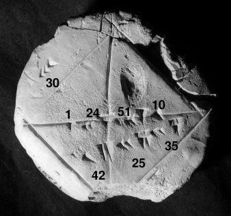
    Babylonian Tablet for 
square root of 2.
 (Wikipedia)

Prediction implies a mechanics, as in knowing a form of a trajectory over time.  Strictly speaking a predictive system implies knowing a solution to the path, set of variable depending on time, time evolution of the system under consideration. Here, we define semi-informally how a prediction system is defined mathematically and show how non-temporal learning can be mapped into a prediction system. 

Temporal learning : Recurrence, trajectory and sequences

A trajectory can be seen as a function of time, identified in recurrence manner. It means $x(t_{i})=f(x_{i-1})$. However, this is one of the possible definitions. The physical equivalent of this appears as a solution to ordinary differential equation, such as the velocity $v(t) = dx(t)/dt$, recurrence on its solution. On the other hand machine learning, an empirical approach is taken and a sequence data such as natural language or a log events occurring in sequence. Any modelling on such data is called temporal learning. This includes classical time-series algorithms, gated units in deep learning and differential equations.

Definition: A prediction system  $\mathscr{F}$ that is build with data $D$ but utilised for a data that is not used in building it $D'$, qualified as such if both $D$ and $D'$ are temporal sets and output of the system is a horizon $\mathbb{H}$, that is a sequence. 

Using non-temporal supervised learning is interpolation or extrapolation

Often practice in industry to turn temporal interactions into flat set of data vectors,  $v_{i}$, $i$ corresponds to a time point or an arbitrary property of the dataset resulting in breaking the temporal associations and causal links.  This could also manifest as set of images with some labels which has no ordering or associational property in the dataset. Even though our system build upon these non-temporal datasets, indeed it constituted a learning systems as interpolation or extrapolation. Their utility in using them for $D'$, strictly speaking does not qualify as prediction systems. 

Mapping with pre-processing

A mapping indeed possible from non-temporal data to a temporal one, if their original form is not in temporal form yet. This is been studied in complexity literature. This requires an algorithm to map flattened data vectors we mentioned into a sequence data. 

Mapping with Causality

A distinct models from causal inference are qualified as predictive systems even if they are trained on non-temporal data, because causality establishes a temporal learning.

Non-temporal modals: Do they still learn?

Even though, we exclude non-temporal model utilisation as non-predictive systems, they still classified as learned models. Because their outputs are generated by a learning procedure. 

Conclusion

Differentiation among temporal and non-temporal learning is provided in associational manner. This results into definition of a prediction system, that excludes non-temporal machine learning models: such as models for unlinked set of vectors, a set of numbers mapped from any data modality. 

Further reading & postscript notes

• Practice causal inference: Conventional supervised learning can't do inference
• Causal inference : Editor's selections from the looper repo.
• Causal models usually are not train but validated or so called discovered.

The concept of overgeneralisation and goodness of rank : Overfitting is not about comparing training and test learning curves

Preamble 

    Walt Disney Hall,
Los Angeles  (Wikipedia)

Unfortunately, it is still thought in machine learning classes that overfitting can be detected by comparing training and test learning curves on the single model's performance.  The origins of this misconception is unknown. Looks like an urban legend has been diffused into main practice  and  even in academic works the misconception taken granted. Overfitting's definition appeared to be inherently about comparing complexities of two (or more) models. Models manifest themself as inductive biases modeller or data scientist inform in their tasks. This makes overfitting in reality a Bayesian concept at its core.  It is not about comparing training and test learning curves that if model is following a noise, but pairwise model comparison-testing procedure to select  more plausable belief among our beliefs that has the least information: entities should not be multiplied beyond necessity i.e., Occam's razor. We introduce a new concept in clarifying this practically, goodness of rank to distinguish from well known goodness of fit, and clarify concepts and provide steps to attribute models with overfitted or under-fitted models.

Poorly generalised model : Overgeneralisation or under-generalisation

The practice that is described in machine learning classes, and  practiced in industry that overfitting is about your model following training set closely but fails to generalised in test set. This is not overfitted model but a model that fails to generalise: a phenomena should be called Overgeneralisation (or under-generalisation). 

A procedure to detect overfitted model : Goodness of rank

We have provided complexity based abstract description of model selection procedure, here as complexity ranking: we will repeat this procedure with identification of the overfilled model explicitly.

In the following steps a sketch of an algorithmic recipe for complexity ranking of inductive biases via informal steps, overfitted model identification explicitly:

1. Define a complexity measure $\mathscr{C}$($\mathscr{M}$) over an inductive bias.
2. Define a generalisation measure  $\mathscr{G}$($\mathscr{M}$, $\mathscr{D}$) over and inductive bias and dataset.
3. Select a set of inductive biases, at least-two, $\mathscr{M}_{1}$ and $\mathscr{M}_{2}$.
4. Produce complexity and generalisation measures on ($\mathscr{M}$, $\mathscr{D}$): Here for two inductive biases: $\mathscr{C}_{1}$, $\mathscr{C}_{2}$,   $\mathscr{G}_{1}$, $\mathscr{G}_{2}$.
5. Ranking of  $\mathscr{M}_{1}$ and $\mathscr{M}_{2}$:  $argmax \{ \mathscr{G}_{1}, \mathscr{G}_{2}\}$ and $argmin \{ \mathscr{C}_{1}, \mathscr{C}_{2}\}$ 
6. $\mathscr{M}_{1}$ is an overfitted model compare to $\mathscr{M}_{2}$   if $\mathscr{G}_{1} <= \mathscr{G}_{2}$ and   $\mathscr{C}_{1} \gt \mathscr{C}_{2}$. 
7. $\mathscr{M}_{2}$ is an overfitted model compare to $\mathscr{M}_{1}$ if $\mathscr{G}_{2} <= \mathscr{G}_{1}$ and   $\mathscr{C}_{2} \gt \mathscr{C}_{1}$.
8. $\mathscr{M}_{1}$ is an underfitted model compare to $\mathscr{M}_{2}$   if $\mathscr{G}_{1} < \mathscr{G}_{2}$ and   $\mathscr{C}_{1} < \mathscr{C}_{2}$.
9. $\mathscr{M}_{2}$ is an underfitted model compare to $\mathscr{M}_{1}$   if $\mathscr{G}_{2} < \mathscr{G}_{1}$ and   $\mathscr{C}_{2} < \mathscr{C}_{1}$.

If two model has the same complexity, then much better generalised model should be selected, in this case we can't conclude that either model is overfitted but generalised differently. Remembering that overfitting is about complexity ranking : Goodness of rank.

But overgeneralisation sounded like overfitting, isn't it?

Operationally overgeneralisation and overfitting implies two different things. Overgeneralisation operationally can be detected with a single model. Because, we can measure the generalisation performance of the model alone with data, in statistical literature this is called goodness of fit. Moreover overgeneralisation can also be called under-generalisation, as both implies poor generalisation performance.

However, overfitting implies a model overly performed compare to an other model i.e., model overfits but compare to what? Practically speaking, overgeneralisation can be detected via holdout method, but not overfitting. Overfitting goes beyond goodness of fit to goodness of rank as we provided recipe as pairwise model comparison.

Conclusion

The practice of comparing training and test learning curves for overfitting diffused into machine learning so deeply, the concept is almost always thought a bit in a fuzzy-way, even in distinguished lectures explicitly. Older textbooks and papers correctly identifies overfitting as comparison problem. As a practitioner, if we bear in mind that overfitting is about complexity ranking and it requires more than one model or inductive bias in order to be identified, then we are in better shape in selecting better model. Overfitting can not be detected via data alone on a single model.  

Further reading

Some of the posts, reverse chronological order, that this blog have tried to convey what overfitting entails and its general implications. 

• Overfitting is about complexity ranking of inductive biases : Algorithmic recipe
• Empirical risk minimization is not learning :A mathematical definition of learning and re-understanding of overfitting and Occam's razor in machine learning
• Critical look on why deployed machine learning model performance degrade quickly.
• Bringing back Occam's razor to modern connectionist machine learning.
• Understanding overfitting: an inaccurate meme in Machine Learning

Glossary 

To make things clear, we provide concept definitions.

Generalisation A concept that if model can perform as good as the data it has not seen before, however seen here is a bit vague, it could have seen data points that are close to the data would be better suited in the context of supervised learning as oppose to compositional learning.

Goodness of fit An approach to check if model is generalised well.  

Goodness of rank An approach to check if model is overfitted or under-fitted comparable to other models.

Holdout method A metod to build a model on the portion of available data and measure the goodness of fit on the holdout part of the data, i.e., test and train.

Inductive bias  A set of assumptions data scientist made in building a representation of the real world, this manifest as model and the assumptions that come with a model.

Model  A model is a biased view of the reality from data scientist. Usually appears as a function of observables $X$ and parameters $\Theta$, $f(X, \Theta)$. The different values of $\Theta$ do not constitute a different model.  See also  What is a statistical model?,  Peter McCullagh 

Occam's razor (Principle of parsimony)  A principle that less complex explanation reflects reality better. Entities should not be multiplied beyond necessity.  

Overgeneralisation (Under-generalisation) If we have a good performance on the training set but very bad performance on the test set, model said to overgeneralise or under-generalise; as a result of goodness of fit testing, i.e., comparing learning curves over test and train datasets.

Regularisation An approach to augment model to improve generalisation.

Postscript Notes

Note: Occam’s razor is a ranking problem: Generalisation is not 

The holy grail of machine learning in practice is hold-out methods. We want to make sure that we don’t overgeneralise. However, a misconception has been propagated that overgeneralisation is mistakenly thought of as synonymous with overfitting. Overfitting has a different connotation as ranking different models rather than measuring the generalisation ability of a single model. The generalisation gap between training and test sets is not about Occam’s razor. 

The conditional query fallacy: Applying Bayesian inference from discrete mathematics perspective

Preamble

    The Tilled Field,
Joan Miró
(Wikipedia)

One of the core concepts in data sciences is conditional probabilities, $p(x|y)$ appear as logical description of many of the tasks, such as formulating regression or as a core concept in Bayesian Inference. However, there is operationally no special meaning of a conditional or joint probabilities as their arguments are no more than a compositional event statements. This raise a question: Is there any fundamental relationship between Bayesian Inference and discrete mathematics that is practically relevant to us as practitioners? Since, both topics are based on discrete statements returning a Boolean variables. Unfortunately, the answer to this question is a rabbit hole and probably even an open research.  There is no clearly established connections between discrete mathematics fundamentals and Bayesian Inference.  

Statement mappings as definition of probability 

Statement is a logical description of some events, or set of events. Let's have a semi-formal description of such statements.

Definition: A mathematical or logical statement formed with boolean relationships $\mathscr{R}$ (conjunctions) among set of events $\mathscr{E}$,  so a statement $\mathbb{S}$ is formed with at least a tuple of $\langle \mathscr{R},  \mathscr{E} \rangle$. 

Relationships can be any binary operator and events could explain anything perceptional, i.e., a discretised existence. This is the core discrete mathematics and almost all problems in this domain formed in this setting from defining functions to graph theory. A probability is no exception and definition naturally follows, as so called statement mapping.

Definition: A probability $\mathbb{P}$ is a statement mapping, $\mathbb{P}: \mathbb{S} \rightarrow [0,1]$. 

The interpretation of this definitions that a logical statement is always True if probability is 1 and always False if it is 0. However, having conditionals based on this is not that clear cut.

Conditional Query Fallacy 

A non-commutative statement may imply, reversing the order of statements should not yield to the same filtered set on the data for Bayesian Inference. However, Bayes' theorem would have a fallacy for statement mappings for conditionals in this sense. 

Definition: The conditional query fallacy is defined as one can not update belief in probability, because reversing order of statements in conditional probabilities halts Bayes' update,  i.e., back to back query results into the same dataset for inference.

At first glance, this appears as a Bayes' rule does not support commutative property, practically posterior being equal to likelihood.  However, this fallacy appears to be a notational misdirection. Inference on the filtered dataset back to back constituting a conditional fallacy i.e., when a query language is used to filter data to get A|B and B|A yielding to the same dataset regardless of filtering order. 

Although, in inference with data, likelihood is actually not a conditional probability, strictly speaking and not a filtering operation. It is merely a measure of update rule. We compute likelihood by multiplying values obtained by i.i.d. samples inserted into conjugate prior, a distribution is involved. Hence, the likelihood computationally is not really a reversal of conditional as in $P(A|B)$ written as reversed, $P(B|A)$.  

Outlook

In computing conditional probabilities for Bayesian Inference, our primary assumption is that conditional probabilities; likelihood and posterior are not identical. Discrete mathematics only allows Bayesian updates, if time evolution is explicitly stated with non-commutative statements for conditionals.

Going back to our initial question, indeed there is a deep connection between the fundamentals of discrete mathematics and Bayesian belief update on events as logical statements. The fallacy sounds a trivial error in judgement but (un)fortunately goes into philosophical definitions of probability that simultaneous tracking of time and sample space is not encoded in any of the notations explicitly, making statement filtering definition of probability a bit shaky.

Glossary of concepts

Statement Mapping A given set of mathematical statements mapped into a domain of numbers.

Probability A statement mapping, where domain is $\mathscr{D} = [0,1]$.

Conditional query fallacy Differently put than the above definition. Thinking that two conditional probabilities as reversed statements of each other in Bayesian inference, yields to the same dataset regardless of time-ordering of the queries.

Notes and further reading

• Fallacy is one computes $P(A|B)=P(B|A)$, while filtering results into identical datasets. Correction would be that, one needs to use different sample sizes for reverse statement or compute joints and marginals separately on their own filtered datasets. Use the first filtering sample size in computing the probability not the total.
• Here, discrete mathematics we refer to appears within arguments of probability. The discussion of discrete parameter estimations are a different topic. Gelman discusses this, here.
• Conjunction Fallacy
• Probability Interpretations
• Bayesian rabbit holes: Decoding conditional probability with non-commutative algebra M. Süzen (2022)
• Holes in Bayesian Statistics Gelman-Yao (2021) : This is a beautifully written article. Specially, proposal that context dependence should be used instead of subjective
• John Allen Paulos’s  Innumeracy: Mathematical Illiteracy and Its Consequences, 

• Random House (1988).  Interestingly Paullos mentions fallacies regarding the conditional probabilities. 

  An oldy book on numerical fallacies but goodie.