Differentiating ensembles and sample spaces: Alignment between statistical mechanics and probability theory

Preamble 

Sample space is the primary concept introduced in any probability and statistics books and in papers. However, there needs to be more clarity about what constitutes a sample space in general: there is no explicit distinction between the unique event set and the replica sets. The resolution of this ambiguity lies in the concept of an ensemble.  The concept is first introduced by American theoretical physicist and engineer Gibbs in his book Elementary principle of statistical mechanics.  The primary utility of an ensemble is a mathematical construction that differentiates between samples and how they would form extended objects. 

In this direction, we provide the basics of constructing ensembles in a pedagogically accessible way from sample spaces that clears up a possible misconception. This usage of ensemble prevents the overuse of the term sample space for different things. We introduce some basic formal definitions.

    Figure: Gibbs's book
 introduced the concept of
ensemble (Wikipedia).

What Gibbs's had in mind by constructing statistical ensembles?

A statistical ensemble is a mathematical tool that connects statistical mechanics to thermodynamics. The concept lies in defining microscopic states for molecular dynamics; in statistics and probability, this corresponds to a set of events. Though these events are different at a microscopic level, they are sampled from a single thermodynamics ensemble, a representative of varying material properties or, in general, a set of independent random variables. In dynamics, micro-states samples an ensemble. This simple idea has helped Gibbs to build a mathematical formalism of statistical mechanics companion to Boltzmann's theories.

Differentiating sample space and ensemble in general

The primary confusion in probability theory on what constitutes a samples space is that there is no distinction between primitive events or events composed of primitive events. We call both sets sample space. This terminology easily overlooked in general as we concentrate on events set but not the primitive events set in solving practical problems.   

Definition: A primitive event $\mathscr{e}$ implies a logically distinct unit of experimental realisation that has not composed of any other events.

Definition: A sample space $\mathscr{S}$ is a set formed by all $N$ distinct primitive events $\mathscr{e}_{i}$.  

By this definition, regardless of how many fair coins are used or if a coin toss in a sequence for the experiment, the sample space is always ${H,T}$, because these are the most primitive distinct events a system can have, i.e., a single coin outcomes. However, the statistical ensemble can be different.  For example for two fair coins or coin toss in sequence of length two, corresponding ensemble of system size two reads ${HH, TT, HT, TH}$. Then, the definition of ensemble follows. 

Definition: An ensemble  $\mathscr{E}$ is a set of ordered set of primitive events $\mathscr{e}_{i}$. These event sets can be sampled with replacement but order matters, i.e., $ \{e_{i}, e_{j} \} \ne  \{e_{j}, e_{i} \}$, $i \ne j$.

Our two coin example's ensemble should be formally written as $\mathscr{E}=\{\{H,H\}, \{T,T\}, \{H,T\}, \{T,H\}\}$, as order matters members $HT$ and $TH$ are distinct. Obviously for a single toss ensemble and a sample space will be the same. 

Ergodicity makes the need for differentiation much more clear : Time and ensemble averaging 

The above distinction makes building time and ensemble averaging much easier. The term ensemble averaging is obvious as we know what would be the ensemble set and averaging over this set for a given observable.  Time averaging then could be achieved by curating a much larger set by resampling with replacement from the ensemble. Note that the resulting time-average value would not be unique, as one can generate many different sample sets from the ensemble. However, bear in mind that the definition of how to measure convergence to ergodic regime is not unique.

Conclusion

Even though the distinction we made sounds very obscure,  this alignment between statistical mechanics and probability theory may clarify the conception of ergodic regimes for general practitioners.

Further reading

• Practical understanding of ergodicity.
• A misconception in ergodicity: Identify ergodic regime not ergodic process

Please Cite:

 @misc{suezen22dess, 

     title = {Differentiating ensembles and sample spaces: Alignment between statistical mechanics and probability theory}, 

     howpublished = {\url{https://science-memo.blogspot.com/2022/11/ensembles-probability-theory.html}, 

     author = {Mehmet Süzen},

     year = {2022}

}  

Postscript

• If there are multiple events coming from set of primitive events, compositional outcomes considered to be ensemble not sample space. Sample space is a set that we sample from, either one or multiple times to build an ensemble. Ensemble notion within pure ML context was also noticed by late David J. C. MacKay, in his book Information Theory, Inference and Learning, Cambridge University Press (2003).

Bayesian rabbit holes: Decoding conditional probability with non-commutative algebra

Preamble

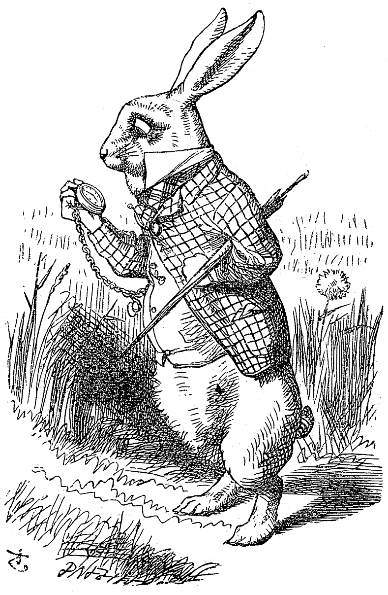
    The White Rabbit
(Wikipedia)

A novice analyst or even experienced (data) scientist would have thought that the bar notation $|$ in representing conditional probability carries some different operational mathematics. Primarily when written in explicit distribution functions $p(x|y)$. Similar approach applies to joint probabilities such as $p(x, y)$ too. One could see a mixture of these, such as $p(x, y | z)$. In this short exposition, we clarify that none of these identifications within arguments of probability do have any different resulting operational meaning. 

Arguments in probabilities: Boolean statement and filtering 

Arguments in any probability are mathematical statements of discrete mathematics that correspond to events in the experimental setting. These are statements declaring some facts with a boolean outcome. These statements are queries to a data set. Such as, if the temperature is above $30$ degrees, $T > 30$. Temperature $T$ is a random variable. Unfortunately, the term random variable is often used differently in many textbooks. It is defined as a mapping rather than as a single variable. The bar $|$ in conditional probability $p(x|y)$, implies statement $x$ given that statement $y$ has already occurred, i.e., if. This interpretation implies that $y$ first occurred before $x$, but it doesn't imply that they are causally linked. The condition plays a role in filtering, a where clause in query languages. $p(x|y)$ boils down to $p_{y}(x)$, where the first statement $y$ is applied to the dataset before computing the probability on the remaining statement $x$.

In the case of joint probabilities $p(x, y)$, events co-occur, i.e., AND statement. In summary, anything in the argument of $p$ is written as a mathematical statement. In the case of assigning a distribution or a functional form to $p$, there is no particular role for conditionals or joints; the modelling approach sets an appropriate structure.

Conditioning does not imply casual direction: do-Calculus do

A filtering interpretation of conditional $p(x|y)$ does not imply causal direction, but $do$ operator does, $p(x|do(y))$. 

Non-commutative algebra: When frequentist are equivalent to Bayesian

Most of the simple filtering operations would result in identical results if reversed. $p(x|y) = p(y|x)$, prior being equal to posterior. This remark implies we can't apply Bayesian learning with commutative statements. We need non-commutative statements; as a result, one can do Bayesian learning with the newly arriving data, i.e., the arrival of new subjective evidence. The reason seems to be due to the frequentist nature of filtering.

Outlook 

Even though we provided some revelations on decoding the operational meaning of conditional probabilities, we suggested that any conditional, joint or any combination of these within the argument of probabilities has no operational purpose other than pre-processing steps. However, the philosophical and practical implications of probabilistic reasoning are always counterintuitive. Probabilistic reasoning is a complex problem computationally. From a causal inference perspective, we are better equipped to tackle these issues with do-Bayesian analysis.  

Further reading

• Discrete Mathematics, Oscar Levin
• Causal Inference in Statistics, A Primer, Judea Pearl, Madelyn Glymour, Nicholas P. Jewell
• Indicative Conditionals Stanford Encyclopedia of Philosophy 
• Bayesian Epistemology Stanford Encyclopedia of Philosophy 

Please Cite as:

 @misc{suezen22brh, 

     title = {Bayesian rabbit holes: Decoding conditional probability with non-commutative algebra}, 

     howpublished = {\url{https://science-memo.blogspot.com/2022/07/bayesian-conditional-noncommutative.html}}, 

     author = {Mehmet Süzen},

     year = {2022}

}  

Particle approximation to probability density functions: Dirac delta function representation

In the previous post, I have briefly shown the idea of using dirac delta function for discrete data representation. In the second example there, a histogram locations for a given set of points are presented as spike trains, where as heights are somehow given in a second sum. This is hard to follow and visualise, of course if you are not that good in reading formulation with different indexes. Due to pedagocial reasons, an easier representation of arbitrary probability density function (PDF), $p(x)$, one would simply need to couple each discrete points with a corresponding weight.

Hence, a set  $\{x_{i}, \omega^{i}\}_{i=1}^{N}$ would be an estimation of PDF, $\hat{p}(x)$ . At this point we can invoke dirac delta function,

$ \hat{p}(x) = \sum_{i=1}^{N} \omega^{i} \delta(x-x_{i})$

Let's revisit the R code given there, this time let's draw uniform numbers between $[-2, 2]$ to get 100  $x_{i}$ values. Simply these numbers will indicate the locations on the x-axis, a spike train.  For simplicity, let's use Gausian distribution for target PDF, $ \mathcal{N}(0, 1)$.  Than, for weights we need to draw numbers using the spike locations. This approach is easier to understand compare to my previous double index notation.

R Example code

Above explained procedure is trivial to implement in R.

1 2 3 4 5 6 7 8 9 10

# Generate locations 100 x locations # out out 1000 points in [-2.0, 2.0] set.seed(42) # Domain where Dirac comb operates Xj = seq(-2,2,0.002) Xi = sample(Xj, 100) # Now generate weights from N(0,1) at those given locations Wi = dnorm(Xi) # Now visualise plot(Xi, Wi, type="h",xlim=c(-2.0,2.0),ylim=c(0,0.6),lwd=2,col="blue",ylab="p")

Conclusion

Above notation introduces second  abuse of notation while actually there must be a secondary regular grid that pics $x_{i}$ values using dirac delta in practice. Because, the argument of $\hat{p}(x)$, is in the discrete domain. So a little better notation that reflects the above code would be

$ \hat{p}(x_j) = \sum_{i=1}^{N} \omega^{i} \delta(x_{j}-x_{i})$

The set $x_j$ is simply defined in a certain domain, for example regularly. Hence I only recommend not to introduce dirac delta for explaining a particle approximation to PDFs for novice students in the class. It will only confuse them even more.

Figure: Spike trains with weights $\hat{p}(x) = \sum_{i=1}^{N} \omega^{i} \delta(x-x_{i})$

Imputation of missing data: Recursive 1D discrete KNN algorithm

Any generated data is often have missing components or values. Probably, the most common occurrence manifest in time series data where there is no value available on the given time point, hence a NaN is placed in general (or NA in R). There is a large literature on how a statistical analysis must be performed in such data sets. For example, a seminal book by Little & Rubin called Statistical Analysis With Missing Data provides very detailed exposure to the field. Probably the simplest of all methods is called imputation. For example there are high quality R packages like imputation or mi that does the job for you. Similarly knnimpute from MATLAB bioinformatics toolbox provides similar solution.
  
k-nearest neighbour algorithm (KNN) is the most common approach to discover the closest available value in the data vector. However, often implementations of KNN contains a lot of options that are not needed for simple imputations in 1D and Euclidean metric. Here I propose 1D discrete KNN recursive algorithm that scans a given vector and determines the closest available value to given index). The main idea is assuming periodic boundary conditions for the vector index boundaries (Two-way linear search on the ring, see simple sketch). This is an $O(\bf{N})$ algorithm, we scan the vector twice in the worst case scenario. I have implemented this idea in MATLAB, for a given matrix. Files are available on the matworks file exchange [link]. This tool could be useful in imputing data in regression design matrices.