Why the simplest explanation is always the best

Preamble

The simplest explanation is always the best among the explanations that are representative.  It is called the principle of parsimony,  Occam's razor. It is the bedrock of scientific enlightenment. There is a recent development that people start to do a category error to discard this principle based on the following setting that lead to misunderstanding: if we say that the simplest model that can explain the data in one representation but another representation requires a more complex model, then we are choosing more complex model. This is obviously wrong. The simplest explanation is to be chosen from the models that captures the complexity on the given representations, not the simplest over both representations. Filter explanations first based on representations then selection follows. Here we shown the core idea via an illustrative example. 

Figure: Circle has a zero Pearson
correlation. (Wikipedia)

Revisiting Occam’s Razor: A case of correlation and geometry

In order to understand this category error, we will work on a concrete example. Let's say we have a data, which is a circular shape $\mathscr{D}(x, y)$, as in figure. We have 3 models: 

$$\mathscr{M}_{1} : y = a x + b $$

$$\mathscr{M}_{2} : y = \sqrt{1-x^{2}} $$

$$\mathscr{M}_{3} : y ~ NN(x)  $$

And $\mathscr{U}$ a utility function, Pearson correlation $C(x, y)$.  We consider performance measure in ranking for the utility and a measure of representation. $\mathscr{M}_{3}$ is a neural network with a lot of parameters.

There is no error in choosing $\mathscr{M}_{1}$ based on the similar correlations these models produce. Principle of parsimony is not violated at all.  This is correct if we are only considering numerical representation. Pearson correlation as a utility works well for purely numerical representation. What about geometric representation? Then we need to change our utility function (representation measure or performance function). 

Let's say if we use curvature as a utility, $\kappa(x,y)$, in this case $\mathscr{M}_{1}$ fails to capture curvature and its is filtered out before Occam's razor can be applied. Then we left with  $\mathscr{M}_{2}$ and $\mathscr{M}_{3}$ . 

Correlation and geometric explanations are two different things. Two vastly different geometries can produce the same correlations.  A model can be quite good in explaining correlation but fails to capture geometric complexity. In this setting, it does not mean that Occam's razor is wrong. We need to apply Occam's razor across representations: numeric, geometric, algebraic, or symbolic, depending on the purpose. Always keep in mind the purpose or utility of model when invoking Occam's razor. Simplest explanation over the required representations that are relevant are the best. 

On the utility, performance and representations measure

Performance function, representation measure and utility functions can be different in real life, here for illustration purposes we consider them interchangeably. 

Conclusion

Nature minimises cost over complexity but under utility constraints. Minimal cost without satisfying utility or representation measure won't be chosen despite being the simplest. We need to filter first based on utility or representation measure before applying Occam's razor. The simplest explanation is always the best among the explanations that are representative. 

 Cite as 

 @misc{suzen25occam, 

     title = { Why the simplest explanation is always the best}, 

     howpublished = {\url{https://science-memo.blogspot.com/2025/11/simplest-explanation-always-best.html}}, 

     author = {Mehmet Süzen},

     year = {2025}

}  

Resolution of misconception of overfitting: Differentiating learning curves from Occam curves

Preamble 

Occam (Wikipedia)

A misconception that overfitted model can be identified with the  amount of generalisation gap between model's training and test sets over its learning curves is still out there. Even in some prominent online lectures and blog posts, this misconception is now repeated without critical look. In general, this practice unfortunately diffuse into some academic papers and industrial,  practitioners attribute poor generalisation to overfitting. We have provided a resolution of this via a new conceptual identification of complexity plots, so called Occam's curves differentiating from a learning curve. An accessible mathematical definitions here will clarify the resolution of the confusion.   

Learning Curve Setting: Generalisation Gap 

Learning curves explain how a given algorithm's generalisation improves over time or experience, originating from Ebbinghaus's work on human memory.  We use inductive bias to express a model, as model can manifest itself in different forms from differential equations to deep learning.

Definition: Given inductive bias $\mathscr{M}$ formed by $n$ datasets with monotonically increasing sizes  $\mathbb{T} = \{|\mathbb{T}_{0}| > |\mathbb{T}_{1}| > ...> |\mathbb{T}_{n}| \}$. A learning curve $\mathscr{L}$ for $\mathscr{M}$ is expressed by the performance measure of the model over datasets,  $\mathbb{p} = \{ p_{0},  p_{1}, ... p_{n} \}$, hence $\mathscr{L}$ is a curve on the plane of $(\mathbb{T}, p)$.  

By this definition, we deduce that $\mathscr{M}$ learns if $\mathscr{L}$ increases monotonically. 

A generalisation gap is defined as follows. 

Definition: Generalisation gap for inductive bias $\mathscr{M}$ is the difference between its' learning curve $\mathscr{L}$ and the learning curve of the unseen datasets, i.e., so-called training, $\mathscr{L}^{train}$. The difference can be simple difference, or a measure differentiating the gap.

We conjecture the following. 

Conjecture: Generalisation gap can't identify if $\mathscr{M}$ is an overfitted model. Overfitting is about Occam's razor, and requires a pairwise comparison between two inductive biases of different complexities.

As conjecture suggests that generalisation gap is not about overfitting, despite the common misconception. Then, why the misconception? The misconception lies on the confusion of how to produce the curve that we could judge overfitting. 

Occam Curves: Overfitting Gap [Occam's Gap] 

In the case of generating Occam curves, a complexity measure  $\mathscr{C}$  over different inductive biases $\mathscr{M_{i}}$ plays a role. Then the definition reads. 

Definition: Given $m$ inductive bias $\mathscr{M_{i}}$ formed by $n$ datasets with monotonically increasing sizes  $\mathbb{T} = \{|\mathbb{T}_{0}| > |\mathbb{T}_{1}| > ...> |\mathbb{T}_{n}| \}$. An Occam curve $\mathscr{O}$ for a given $\mathscr{M}$ is expressed by the performance measure of the model over complexity-dataset size points  $\mathbb{F} = [(|\mathbb{T}_{0}|, \mathscr{C}),  (|\mathbb{T}_{1}| , \mathscr{C}), ...,  (|\mathbb{T}_{n}| , \mathscr{C}) ] $; Performance of a given inductive bias reads $\mathbb{p} = \{ p_{0},  p_{1}, ... p_{n} \}$, hence Occam curve, $\mathscr{O}$ is a curve on the plane of $(\mathbb{F}, p)$.  

 

Given definition, producing Occam curves are more complicated than simply plotting test and train curves over batches. The ordering in $\mathbb{F}$ forms what is so-called goodness of rank.

Summary and take home

Resolution of misconception of overfitting lies in producing Occam curves to judge the bias-variance tradeoff, not the learning curves of a single model. 

Further reading & notes

• Further posts and a glossary : The concept of overgeneralisation and goodness of rank.
• Double decent phenomenon, it uses Occam's curves, not learning curves.
• We use dataset size as an interpretation of increasing experience, there could be other ways of expressing a gained experience, but we take the most obvious evidence.

Please cite as follows:

 @misc{suezen23rmo, 

     title = {Resolution of misconception of overfitting: Differentiating learning curves from Occam curves}, 

     howpublished = {\url{https://science-memo.blogspot.com/2023/04/Occam-curves.html}}, 

     author = {Mehmet Süzen},

     year = {2023}

}  

Postscript notes

Take home messages

Understanding Generalisation Gap and Occam’s gap

Model selection and evaluations are usually confused by novice and as well as experienced data scientists and professionals doing modelling. There are a lot of misconceptions in the literature, but in practice primary take home messages can be summarised as follows:

1. What is a model? A model is an “inductive bias” of the modeller, a selected parametrised functions for example, a neural network architecture choice. Contrary to many, specific parametrisation of a model (deep learning architecture) is not a different model.
2. A model’s test and training performance difference is about generalisation gap. Overfitting and under-fitting is not about generalisation gap.
3. Overfitting or under-fitting is a comparison problem: How a model deviates from a reference model? This is called Occam’s gap or so called model selection error.
4. Occam’s gap generalises Empirical Risk minimisation over a learning curve.  Empirical risk minimisation itself is not about learning.

How and when a model generalises well and generalisation of empirical risk minimisation are currently an open research topics.

Misconceptions on non-temporal learning: When do machine learning models qualify as prediction systems?

Preamble

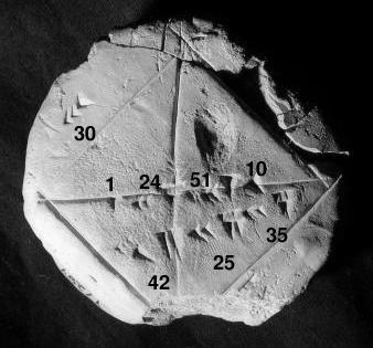
    Babylonian Tablet for 
square root of 2.
 (Wikipedia)

Prediction implies a mechanics, as in knowing a form of a trajectory over time.  Strictly speaking a predictive system implies knowing a solution to the path, set of variable depending on time, time evolution of the system under consideration. Here, we define semi-informally how a prediction system is defined mathematically and show how non-temporal learning can be mapped into a prediction system. 

Temporal learning : Recurrence, trajectory and sequences

A trajectory can be seen as a function of time, identified in recurrence manner. It means $x(t_{i})=f(x_{i-1})$. However, this is one of the possible definitions. The physical equivalent of this appears as a solution to ordinary differential equation, such as the velocity $v(t) = dx(t)/dt$, recurrence on its solution. On the other hand machine learning, an empirical approach is taken and a sequence data such as natural language or a log events occurring in sequence. Any modelling on such data is called temporal learning. This includes classical time-series algorithms, gated units in deep learning and differential equations.

Definition: A prediction system  $\mathscr{F}$ that is build with data $D$ but utilised for a data that is not used in building it $D'$, qualified as such if both $D$ and $D'$ are temporal sets and output of the system is a horizon $\mathbb{H}$, that is a sequence. 

Using non-temporal supervised learning is interpolation or extrapolation

Often practice in industry to turn temporal interactions into flat set of data vectors,  $v_{i}$, $i$ corresponds to a time point or an arbitrary property of the dataset resulting in breaking the temporal associations and causal links.  This could also manifest as set of images with some labels which has no ordering or associational property in the dataset. Even though our system build upon these non-temporal datasets, indeed it constituted a learning systems as interpolation or extrapolation. Their utility in using them for $D'$, strictly speaking does not qualify as prediction systems. 

Mapping with pre-processing

A mapping indeed possible from non-temporal data to a temporal one, if their original form is not in temporal form yet. This is been studied in complexity literature. This requires an algorithm to map flattened data vectors we mentioned into a sequence data. 

Mapping with Causality

A distinct models from causal inference are qualified as predictive systems even if they are trained on non-temporal data, because causality establishes a temporal learning.

Non-temporal modals: Do they still learn?

Even though, we exclude non-temporal model utilisation as non-predictive systems, they still classified as learned models. Because their outputs are generated by a learning procedure. 

Conclusion

Differentiation among temporal and non-temporal learning is provided in associational manner. This results into definition of a prediction system, that excludes non-temporal machine learning models: such as models for unlinked set of vectors, a set of numbers mapped from any data modality. 

Further reading & postscript notes

• Practice causal inference: Conventional supervised learning can't do inference
• Causal inference : Editor's selections from the looper repo.
• Causal models usually are not train but validated or so called discovered.

The concept of overgeneralisation and goodness of rank : Overfitting is not about comparing training and test learning curves

Preamble 

    Walt Disney Hall,
Los Angeles  (Wikipedia)

Unfortunately, it is still thought in machine learning classes that overfitting can be detected by comparing training and test learning curves on the single model's performance.  The origins of this misconception is unknown. Looks like an urban legend has been diffused into main practice  and  even in academic works the misconception taken granted. Overfitting's definition appeared to be inherently about comparing complexities of two (or more) models. Models manifest themself as inductive biases modeller or data scientist inform in their tasks. This makes overfitting in reality a Bayesian concept at its core.  It is not about comparing training and test learning curves that if model is following a noise, but pairwise model comparison-testing procedure to select  more plausable belief among our beliefs that has the least information: entities should not be multiplied beyond necessity i.e., Occam's razor. We introduce a new concept in clarifying this practically, goodness of rank to distinguish from well known goodness of fit, and clarify concepts and provide steps to attribute models with overfitted or under-fitted models.

Poorly generalised model : Overgeneralisation or under-generalisation

The practice that is described in machine learning classes, and  practiced in industry that overfitting is about your model following training set closely but fails to generalised in test set. This is not overfitted model but a model that fails to generalise: a phenomena should be called Overgeneralisation (or under-generalisation). 

A procedure to detect overfitted model : Goodness of rank

We have provided complexity based abstract description of model selection procedure, here as complexity ranking: we will repeat this procedure with identification of the overfilled model explicitly.

In the following steps a sketch of an algorithmic recipe for complexity ranking of inductive biases via informal steps, overfitted model identification explicitly:

1. Define a complexity measure $\mathscr{C}$($\mathscr{M}$) over an inductive bias.
2. Define a generalisation measure  $\mathscr{G}$($\mathscr{M}$, $\mathscr{D}$) over and inductive bias and dataset.
3. Select a set of inductive biases, at least-two, $\mathscr{M}_{1}$ and $\mathscr{M}_{2}$.
4. Produce complexity and generalisation measures on ($\mathscr{M}$, $\mathscr{D}$): Here for two inductive biases: $\mathscr{C}_{1}$, $\mathscr{C}_{2}$,   $\mathscr{G}_{1}$, $\mathscr{G}_{2}$.
5. Ranking of  $\mathscr{M}_{1}$ and $\mathscr{M}_{2}$:  $argmax \{ \mathscr{G}_{1}, \mathscr{G}_{2}\}$ and $argmin \{ \mathscr{C}_{1}, \mathscr{C}_{2}\}$ 
6. $\mathscr{M}_{1}$ is an overfitted model compare to $\mathscr{M}_{2}$   if $\mathscr{G}_{1} <= \mathscr{G}_{2}$ and   $\mathscr{C}_{1} \gt \mathscr{C}_{2}$. 
7. $\mathscr{M}_{2}$ is an overfitted model compare to $\mathscr{M}_{1}$ if $\mathscr{G}_{2} <= \mathscr{G}_{1}$ and   $\mathscr{C}_{2} \gt \mathscr{C}_{1}$.
8. $\mathscr{M}_{1}$ is an underfitted model compare to $\mathscr{M}_{2}$   if $\mathscr{G}_{1} < \mathscr{G}_{2}$ and   $\mathscr{C}_{1} < \mathscr{C}_{2}$.
9. $\mathscr{M}_{2}$ is an underfitted model compare to $\mathscr{M}_{1}$   if $\mathscr{G}_{2} < \mathscr{G}_{1}$ and   $\mathscr{C}_{2} < \mathscr{C}_{1}$.

If two model has the same complexity, then much better generalised model should be selected, in this case we can't conclude that either model is overfitted but generalised differently. Remembering that overfitting is about complexity ranking : Goodness of rank.

But overgeneralisation sounded like overfitting, isn't it?

Operationally overgeneralisation and overfitting implies two different things. Overgeneralisation operationally can be detected with a single model. Because, we can measure the generalisation performance of the model alone with data, in statistical literature this is called goodness of fit. Moreover overgeneralisation can also be called under-generalisation, as both implies poor generalisation performance.

However, overfitting implies a model overly performed compare to an other model i.e., model overfits but compare to what? Practically speaking, overgeneralisation can be detected via holdout method, but not overfitting. Overfitting goes beyond goodness of fit to goodness of rank as we provided recipe as pairwise model comparison.

Conclusion

The practice of comparing training and test learning curves for overfitting diffused into machine learning so deeply, the concept is almost always thought a bit in a fuzzy-way, even in distinguished lectures explicitly. Older textbooks and papers correctly identifies overfitting as comparison problem. As a practitioner, if we bear in mind that overfitting is about complexity ranking and it requires more than one model or inductive bias in order to be identified, then we are in better shape in selecting better model. Overfitting can not be detected via data alone on a single model.  

Further reading

Some of the posts, reverse chronological order, that this blog have tried to convey what overfitting entails and its general implications. 

• Overfitting is about complexity ranking of inductive biases : Algorithmic recipe
• Empirical risk minimization is not learning :A mathematical definition of learning and re-understanding of overfitting and Occam's razor in machine learning
• Critical look on why deployed machine learning model performance degrade quickly.
• Bringing back Occam's razor to modern connectionist machine learning.
• Understanding overfitting: an inaccurate meme in Machine Learning

Glossary 

To make things clear, we provide concept definitions.

Generalisation A concept that if model can perform as good as the data it has not seen before, however seen here is a bit vague, it could have seen data points that are close to the data would be better suited in the context of supervised learning as oppose to compositional learning.

Goodness of fit An approach to check if model is generalised well.  

Goodness of rank An approach to check if model is overfitted or under-fitted comparable to other models.

Holdout method A metod to build a model on the portion of available data and measure the goodness of fit on the holdout part of the data, i.e., test and train.

Inductive bias  A set of assumptions data scientist made in building a representation of the real world, this manifest as model and the assumptions that come with a model.

Model  A model is a biased view of the reality from data scientist. Usually appears as a function of observables $X$ and parameters $\Theta$, $f(X, \Theta)$. The different values of $\Theta$ do not constitute a different model.  See also  What is a statistical model?,  Peter McCullagh 

Occam's razor (Principle of parsimony)  A principle that less complex explanation reflects reality better. Entities should not be multiplied beyond necessity.  

Overgeneralisation (Under-generalisation) If we have a good performance on the training set but very bad performance on the test set, model said to overgeneralise or under-generalise; as a result of goodness of fit testing, i.e., comparing learning curves over test and train datasets.

Regularisation An approach to augment model to improve generalisation.

Postscript Notes

Note: Occam’s razor is a ranking problem: Generalisation is not 

The holy grail of machine learning in practice is hold-out methods. We want to make sure that we don’t overgeneralise. However, a misconception has been propagated that overgeneralisation is mistakenly thought of as synonymous with overfitting. Overfitting has a different connotation as ranking different models rather than measuring the generalisation ability of a single model. The generalisation gap between training and test sets is not about Occam’s razor. 

The conditional query fallacy: Applying Bayesian inference from discrete mathematics perspective

Preamble

    The Tilled Field,
Joan Miró
(Wikipedia)

One of the core concepts in data sciences is conditional probabilities, $p(x|y)$ appear as logical description of many of the tasks, such as formulating regression or as a core concept in Bayesian Inference. However, there is operationally no special meaning of a conditional or joint probabilities as their arguments are no more than a compositional event statements. This raise a question: Is there any fundamental relationship between Bayesian Inference and discrete mathematics that is practically relevant to us as practitioners? Since, both topics are based on discrete statements returning a Boolean variables. Unfortunately, the answer to this question is a rabbit hole and probably even an open research.  There is no clearly established connections between discrete mathematics fundamentals and Bayesian Inference.  

Statement mappings as definition of probability 

Statement is a logical description of some events, or set of events. Let's have a semi-formal description of such statements.

Definition: A mathematical or logical statement formed with boolean relationships $\mathscr{R}$ (conjunctions) among set of events $\mathscr{E}$,  so a statement $\mathbb{S}$ is formed with at least a tuple of $\langle \mathscr{R},  \mathscr{E} \rangle$. 

Relationships can be any binary operator and events could explain anything perceptional, i.e., a discretised existence. This is the core discrete mathematics and almost all problems in this domain formed in this setting from defining functions to graph theory. A probability is no exception and definition naturally follows, as so called statement mapping.

Definition: A probability $\mathbb{P}$ is a statement mapping, $\mathbb{P}: \mathbb{S} \rightarrow [0,1]$. 

The interpretation of this definitions that a logical statement is always True if probability is 1 and always False if it is 0. However, having conditionals based on this is not that clear cut.

Conditional Query Fallacy 

A non-commutative statement may imply, reversing the order of statements should not yield to the same filtered set on the data for Bayesian Inference. However, Bayes' theorem would have a fallacy for statement mappings for conditionals in this sense. 

Definition: The conditional query fallacy is defined as one can not update belief in probability, because reversing order of statements in conditional probabilities halts Bayes' update,  i.e., back to back query results into the same dataset for inference.

At first glance, this appears as a Bayes' rule does not support commutative property, practically posterior being equal to likelihood.  However, this fallacy appears to be a notational misdirection. Inference on the filtered dataset back to back constituting a conditional fallacy i.e., when a query language is used to filter data to get A|B and B|A yielding to the same dataset regardless of filtering order. 

Although, in inference with data, likelihood is actually not a conditional probability, strictly speaking and not a filtering operation. It is merely a measure of update rule. We compute likelihood by multiplying values obtained by i.i.d. samples inserted into conjugate prior, a distribution is involved. Hence, the likelihood computationally is not really a reversal of conditional as in $P(A|B)$ written as reversed, $P(B|A)$.  

Outlook

In computing conditional probabilities for Bayesian Inference, our primary assumption is that conditional probabilities; likelihood and posterior are not identical. Discrete mathematics only allows Bayesian updates, if time evolution is explicitly stated with non-commutative statements for conditionals.

Going back to our initial question, indeed there is a deep connection between the fundamentals of discrete mathematics and Bayesian belief update on events as logical statements. The fallacy sounds a trivial error in judgement but (un)fortunately goes into philosophical definitions of probability that simultaneous tracking of time and sample space is not encoded in any of the notations explicitly, making statement filtering definition of probability a bit shaky.

Glossary of concepts

Statement Mapping A given set of mathematical statements mapped into a domain of numbers.

Probability A statement mapping, where domain is $\mathscr{D} = [0,1]$.

Conditional query fallacy Differently put than the above definition. Thinking that two conditional probabilities as reversed statements of each other in Bayesian inference, yields to the same dataset regardless of time-ordering of the queries.

Notes and further reading

• Fallacy is one computes $P(A|B)=P(B|A)$, while filtering results into identical datasets. Correction would be that, one needs to use different sample sizes for reverse statement or compute joints and marginals separately on their own filtered datasets. Use the first filtering sample size in computing the probability not the total.
• Here, discrete mathematics we refer to appears within arguments of probability. The discussion of discrete parameter estimations are a different topic. Gelman discusses this, here.
• Conjunction Fallacy
• Probability Interpretations
• Bayesian rabbit holes: Decoding conditional probability with non-commutative algebra M. Süzen (2022)
• Holes in Bayesian Statistics Gelman-Yao (2021) : This is a beautifully written article. Specially, proposal that context dependence should be used instead of subjective
• John Allen Paulos’s  Innumeracy: Mathematical Illiteracy and Its Consequences, 

• Random House (1988).  Interestingly Paullos mentions fallacies regarding the conditional probabilities. 

  An oldy book on numerical fallacies but goodie.    

Overfitting is about complexity ranking of inductive biases : Algorithmic recipe

Preamble

    Figure: Moon patterns
human brain
 invents. (Wikipedia)

Detecting overfitting is inherently a comparison problem of the complexity of multiple objects, i.e., models or an algorithm capable of making predictions. A model is overfitted (underfitted) if we only compare it to another model. Model selection involves comparing multiple models with different complexities. The summary of this approach with basic mathematical definitions is given here.

Misconceptions: Poor generalisation is not synonymous with overfitting. 

None of these techniques would prevent us from overfitting: Cross-validation, having more data, early stopping, and comparing test-train learning curves are all about generalisation. Their purpose is not to detect overfitting.

We need at least two different models, i.e., two different inductive biases, to judge which model is overfitted. One distinct approach in deep learning, called dropout, prevents overfitting while it alternates between multiple models, i.e., multiple inductive bias. For judgment, dropout implementation has to compare those alternating model test performances during training to judge overfitting. 

What is an inductive bias? 

There are multiple inceptions of inductive bias. Here, we concentrate on a parametrised model, $\mathscr{M}(\theta)$ on a dataset $\mathscr{D}$, the selection of a model type, or modelling approach, usually manifest as a functional form $\mathscr{M}=f(x)$ or as a function approximation, i.e., for example neural network, are all manifestation of inductive biases. Different parameterisation of model learned on the subsets of the dataset are still the same inductive bias.

Complexity ranking of inductive biases: An Algorithmic recipe 

We are sketching out an algorithmic recipe for complexity ranking of inductive biases via informal steps:

1. Define a complexity measure $\mathscr{C}$($\mathscr{M}$) over an inductive bias.
2. Define a generalisation measure  $\mathscr{G}$($\mathscr{M}$, $\mathscr{D}$) over and inductive bias and dataset.
3. Select a set of inductive biases, at least-two, $\mathscr{M}_{1}$ and $\mathscr{M}_{2}$.
4. Produce complexity and generalisation measures on ($\mathscr{M}$, $\mathscr{D}$): Here for two inductive biases: $\mathscr{C}_{1}$, $\mathscr{C}_{2}$,   $\mathscr{G}_{1}$, $\mathscr{G}_{2}$.
5. Ranking of  $\mathscr{M}_{1}$ and $\mathscr{M}_{2}$:  $argmax \{ \mathscr{G}_{1}, \mathscr{G}_{2}\}$ and $argmin \{ \mathscr{C}_{1}, \mathscr{C}_{2}\}$

The core concept appears as when generalisations are close enough we pick out the inductive bias that is less complex. 

Conclusion & Outlook

In practice,  probably due to hectic delivery constraints, or mere laziness, we still rely on simple holdout method to build models, only single test and train split, not even learning curves, specially in deep learning models without practicing Occam's razor. A major insight in this direction appears to be that, holdout approach can only help us to detect generalisation, not overfitting. We clarify this via the concept of inductive bias distinguishing that different parametrisation of the same model doesn't change the inductive bias introduced by the modelling choice. 

In fact, due to resource constraints of model life-cycle, i.e., energy consumption and cognitive load of introducing a complex model, practicing proper Occam's razor: complexity ranking of inductive biases, is much more important than ever for sustainable environment and human capital.

Further reading

Some of the posts, reverse chronological order, that this blog have tried to convey what overfitting entails and its general implications. 

• Empirical risk minimization is not learning :A mathematical definition of learning and re-understanding of overfitting and Occam's razor in machine learning
• Critical look on why deployed machine learning model performance degrade quickly.
• Bringing back Occam's razor to modern connectionist machine learning.
• Understanding overfitting: an inaccurate meme in Machine Learning

Empirical risk minimization is not learning : A mathematical definition of learning and re-understanding of overfitting and Occam's razor in machine learning

    Simionescu Function (Wikipedia)

Preamble

The holy grail of machine learning appears to be the empirical risk minimisation. However, on the contrary to general dogma,  the primary objective of machine learning is not risk minimisation per se but mimicking human or animal learning. Empirical risk minimisation is just a snap-shot in this direction and is part of a learning measure, not the primary objective.

Unfortunately, all current major machine learning libraries are implementing empirical risk minimisation as primary objective, so called a training, manifest as usually .fit. Here we provide a mathematical definition of learning in the language of empirical risk minimisation and its implications on two very important concepts, overfitting and Occam's razor.

Our exposition is still informal but it should be readable for experienced practitioners.

Definition: Empirical Risk Minimization

Given set of $k$ observation $\mathscr{O} = \{o_{1}, ..., o_{k} \}$ where $o_{i} \in \mathbb{R}^{n}$, $n$-dimensional vectors.  Corresponding labels or binary classes, the set $\mathscr{S} = \{ s_{1}, .., s_{k}\}$, with $s_{i} \in \{0,1\}$ is defined. A function $g$  maps observations to classes $g: \mathscr{O} \to \mathscr{S}$.  An error function (or loss) $E$ measures the error made by the estimated map function $\hat{g}$ compare to true map function $g$,  $E=E(\hat{g}, g)$.  The entire idea of supervised machine learning boils down to minimising a functional called ER (Empirical Risk), here we denoted by $G$, it is a functional, meaning is a function of function, over the domain $\mathscr{D} = Tr(\mathscr{O} x \mathscr{S})$ in discrete form, $$ G[E] = \frac{1}{k} {\Large \Sigma}_{\mathscr{D} }  E(\hat{g}, g) $$.  This is so called a training a machine learning model, or an estimation for  $\hat{g}$. However, testing this estimate on the new data is not the main purpose of the learning.

Definition: Learning measure 

A learning measures $M$, on $\hat{g}$ is defined over set of $l$ observations with increasing size, $\Theta = \{ \mathscr{O}_{1}, ..., \mathscr{O}_{l}\}$ whereby size of each set is monotonically higher, meaning that $ | \mathscr{O}_{1}| < | \mathscr{O}_{2}| , ...,< | \mathscr{O}_{l}|$.

Definition: Empirical Risk Minimization with a learning measure (ERL)

Now, we are in a position to reformulate ER with learning measure, we call this ERL. This come with a testing procedure.

If empirical risks $G[E_{j}]$ lowers monotonically, $ G[E_{1}] > G[E_{2}] > ... > G[E_{l}]$, then we said the functional form of $\hat{g}$ is a learning over the set  $\Theta$.  

Functional form of $\hat{g}$ : Inductive bias

The functional form implies a model selection, and a technical term of this also known as inductive bias with other assumptions, meaning the selection of complexity of the model, for example a linear regression or nonlinear regression.

Re-understanding of overfitting and Occam's razor from ERL perspective 

If we have two different ERLs on $\hat{g}^{1}$ and $\hat{g}^{2}$. Then overfitting is a comparison problem between monotonically increasing empirical risks. If model, here an inductive bias or a functional form, over learning measure, we select the one with "higher monotonicity" and the less complex one and call the other overfitted model. Complexity here boils down to functional complexity of $\hat{g}^{1}$ and  $\hat{g}^{2}$  and overfitting can only be tested with two models over monotonicity (increasing) of ERLs.

Conclusions

In the age of deep learning systems, the classical learning theory needs an update on how do we define what is learning beyond a single shot fitting exercise. A first step in this direction would be to improve upon basic definitions of Empirical Risk (ER) minimisation that would reflect real-life learning systems similar to forgetting mechanism proposed by Ebbinghaus. This is consistent with Tom Mitchell's definition of operational machine learning. A next level would be to add causality in the definition.

Please cite as follows:

 @misc{suezen22erm, 

     title = { Empirical risk minimization is not learning : A mathematical definition of learning and re-understanding of overfitting and Occam's razor in machine learning}, 

     howpublished = {\url{http://science-memo.blogspot.com/2022/06/empirical-risk-minimisation-learning-curve.html}}, 

     author = {Mehmet Süzen},

     year = {2022}

}  

Postscript Notes

Following notes are added after initial release 

Postscript 1: Understanding overfitting as comparison of inductive biases

ERM could be confusing for even experienced researchers. It is indeed about risk measure. We measure the risk of a model, i.e., machine learning procedure that how much error would it make on the  given new data distribution, as in risk of investing. This is quite a similar notion as in financial risk of loss but not explicitly stated. 

Moreover, a primary objective of machine learning is not ERM but measure learning curves and pair-wise comparison of  inductive biases, avoiding overfitting.  An inductive bias, here we restrict the concept as in model  type,  is a model selection step: different  parametrisation of the same model are still the same inductive bias.  That’s why standard training-error learning curves can’t be used to detect overfitting alone. 

Postscript 2: Learning is not to optimise: Thermodynamic limit, true risk and accessible learning space

True risk minimisation in machine learning is not possible, instead we rely on ERM, i.e., Emprical Risk Minimisation.  However, the purpose of machine learning algorithm is not to minimise risk, as we only have a  partial knowledge about the reality through data.  Learning implies finding out a region  in accessible learning space whereby there is a monotonic increase in the objective; ERM is only a single point on this space, the concept rooted in German scientist Hermann Ebbinghaus  work on memory.

There is an intimate connection to thermodynamic limit and true risk in this direction as an open research.  However, it doesn’t imply infinite limit of data, but the observable’s behaviour. That’s why full empiricist approaches usually requires a complement of a physical laws,  such as Physics Informed Neural Networks (PINNs) or Structural Causal Model (SCM).

Postscript 3: Missing abstraction in modern machine learning libraries 

Interestingly current modern machine learning libraries stop abstracting further than fitting: .fit and .predict. This is short of learning as in machine learning. Learning manifest itself In learning curves. .learn functionality can be leveraged beyond fitting and if we are learning via monotonically increasing performance. Origin of this lack of tools for .learn appears to be how Empirical Risk Minimisation (ERM) is formulated on a single task.

Physics origins of the most important statistical ideas of recent times

Figure: Maxwell's handwritings, 
state diagram (Wikipedia)

Preamble

The modern statistics now move into an emerging field called data science that amalgamate many different fields from high performance computing to control engineering. However, the emergent behaviour from researchers in machine learning and statistics that, sometimes they omit naïvely and probably unknowingly the fact that some of the most important ideas in data sciences are actually originated from Physics discoveries and specifically developed by physicist. In this short exposition we try to review these physics origins on the areas defined by Gelman and Vehtari (doi). Additional section is also added in other possible areas that are currently the focus of active research in data sciences. 

Bootstrapping and simulation based inference : Gibbs's Ensemble theory and Metropolis's simulations

Bootstrapping is a novel idea of estimations with uncertainty with given set of samples. It is mostly popularised by Efron and his contribution is immense, making this tool available to all researchers doing quantitative analysis.  However, the origins of bootstrapping can be traced back to the idea of ensembles in statistical physics, which is introduced by J. Gibbs. The ensembles in physics allow us to do just what bootstrapping helps, estimating a quantity of interest with sub-sampling, in the case of statistical physics this appears as sampling a set of different microstates. Using this idea Metropolis devised a inference in 1953, to compute ensemble averages for liquids using computers.  Note that, usage of Monte Carlo approach for pure mathematical nature, i.e., solving integrals, appear much earlier with von Neumann's efforts.

Causality : Hamiltonian systems to Thermodynamic potentials

Figure: Maxwell 
Relations as causal
diagrams.

Even though the historical roots of causal analysis in early 20th century attributed to Wright 1923 for his definition of path analysis, causality was the core tanents of Newtonian mechanics in distinguishing left and right of the equations of motions in the form of differential equations, and the set of differential equations following that with Hamiltonian Mechanics is actually forms a graph, i.e., relationships between generalised coordinates, momentum and positions. This connection is never acknowledge in early statistical literature, and probably causal constructions from classical physics were not well known in that community or did not find its way to data-driven mechanics. Similarly, causal construction of thermodynamic potentials appear as a directed graph as in, Born wheel. It appears as a mnemonic but it is actually  causally constructed via Legendre Transformations.  Of course, causality, philosophically speaking, is discussed since Ancient Greece but here we restrict the discussion on solely quantitative theories after Newton.

Overparametrised models and regularisation : Poincaré classifications and astrophysical dynamics

The current deep learning systems classified as massively overparametrized systems. However, the lower dimensional understanding of this phenomenon were well studied by Poincare's classification of classical dynamics, namely the measurement problem of having overdetermined system of differential equations, i.e., whereby inverse problems are well known in astrophysics and theoretical mechanics.     

High-performance computing: Big-data to GPUs

Similarly, using supercomputers or as now we call it high-performance computation with big data generating processes were actually can be traced back to Manhattan project and ENIAC that aims solving scattering equations and almost 50 years of development on this direction before 2000s. 

Conclusion

The impressive development of new emergent field of data science as a larger perspective of statistics into computer science have strong origins from core Physics literature and research. These connections are not sufficiently cited or acknowledged. Our aim in this short exposition is to bring these aspects into the attention of data science practitioners and researchers alike.

Further reading

Some of the mentioned works and related reading list, papers or books.

• What are the Most Important Statistical Ideas of the Past 50 Years? Gelman & Vehtari (2021)
• Leisurely Look at the Bootstrap, the Jackknife, and Cross-Validation, Bradley Efron and Gail Gong (1983)
• Elementary Principles in Statistical Mechanics, Gibbs (1902)
• Equation of State Calculations by Fast Computing Machines, Metropolis et. al. (1953)
• Generalized statistical mechanics: connection with thermodynamics, Curado-Tsallis (1992)
• Poincaré sections of Hamiltonian systems (1996)

• Statistical mechanics of ensemble learning, Anders Krogh and Peter Sollich (1997)

Please cite as follows:

 @misc{suezen22pom, 

     title = { Physics origins of the most important statistical ideas of recent times }, 

     howpublished = {\url{http://science-memo.blogspot.com/2022/02/physics-origins-of-most-important.html}, 

     author = {Mehmet Süzen},

     year = {2022}

  }

Appendix: Pearson correlation and Lattices

Auguste Bravais is famous for his contribution in foundational work on the mathematical theory for crystallography, now seems to be going far beyond periodic solids. Unknown to many, he actually first driven the expression for what we know today as correlation coefficient or  Pearson’s correlation or less commonly Pearson-Galton coefficient. Interestingly, one of the grandfathers of causal analysis Wright is mentioned this in his seminal work of 1921 titled “Correlation and causation” acknowledged Bravais for his 1849 work as the first derivation of correlation.

Appendix: Partition function and set theoretic probability

Long before Kolmogorov set forward his formal foundations of probabilities, Boltzmann, Maxwell and Gibbs build theories of statistical mechanics using probabilistic language and even define settings for set theoretic foundations by introducing ensembles for thermodynamics. For example, partition function (Z) appeared as defining a normalisation factor that summation of densities should yield to 1. Apparently Kolmogorov and contemporaries inspired a lot from physics and mechanics literature.

Appendix: Generative AI

Of course now generative AI took over the hype. Indeed physics of diffusion from Fokker-Planck equation to basic Langevin dynamics is leveraged.  

 

Appendix: Physics is fundamental for the advancement of AI research and practice 

AI as a phenomena appears to be in the domain of core physics. For this reason, studying physics as a (post)-degree or as a self-study modules will give students and practitioners alike a definitive cutting-edge insights.  

• Statistical models based on correlations originates from physics of periodic solids and astrophysical n-body dynamics.
• Neural networks originates from the modelling magnetic materials in discrete states and later named as cooperative phenomenon. Their training dynamics closely follows free-energy minimisation.
• Causality roots in ensemble theory of physical entropy.
• Almost all sampling based techniques are based on the idea of sampling  physics of energy surfaces, i.e. Potential Energy Surfaces. (PES).
• Generative AI  originates from physics of diffusion of fluids: classical  Liouville description of the classical mechanics, i.e, phase-space flows and generalised Fokker-Planck dynamics. 
• Language models based on attention are actually coarse-grained entropy-dynamics
  introduced by Gibbs: ‘Attention Layers’ behaves as coarse-graining procedure, i.e, compressed
  causal graphs mapping.

This is not about building analogies to physics but as foundational topics to AI.