Showing posts with label statistical mechanics. Show all posts

Tuesday, 3 June 2025

Compressive algorithmic randomness:
Gibbs-randomness proposition for massively energy efficient deep learning

Figure: Dual Tomographic Compression
Performance, Süzen, 2025.
Preamble

Randomness is elusive and its probably one of the outstanding concepts for human scientific endeavour, along with gravity. Kolmogorov complexity, appears to be so novel in trying to answering "what is randomness?". The idea that the length of the smallest model that can generate the random sequence determines its complexity was a turning point in history of science. Similarly, it implies choosing the simplest model for explaining a phenomenon. That's why Kolmogorov's work was also supported by the ideas of Solomonoff and Chaitin. A recent work, explores this algorithmic information from compression perspective with Gibbs entropy.

A strange tale of path from applied research to fundamental proposition. 

During study of model compression algorithm development, I have noticed an amazing behaviour that information, entropy and compression over compression process have a more in depth. 

New concepts in compression and randomness via train-compress cycles

Here, we explain the new concepts for both deep learning model compression and on the interplay between compression and algorithmic randomness.

Inverse compressed sensing (iCS): Normally CS procedure is applied to reconstruct an unknown signal with fewer measurements. In the case of deep learning train-compress, weights are known at one point in the training cycle. If we create hypothetical measurements, using CS formulations, we can reconstruct weights sparse projection. 

Dual Tomographic Compression: Applying iCS for the input and output of neuronal level, layer-wise, simultaneously.  

Weight rays:  An output reconstructed vector out of DTC; weights given sparsity level, though they are not generated in isolation but within train-compress cycle.

Gibbs randomness proposition : An extension of Kolmogorov complexity for a compression process. That, directed randomness is the same as complexity reduction, i.e., compression. 

Conclusion 

A new technique called DTC can be used to train deep learning with model compression on the fly. This gives rise to massively energy efficient deep learning, reaching almost ~98% reduction in energy use.  Moreover, the technique also demonstrated an extended version of Kolmogorov complexity. 

Further reading 

Paper & codes are released :


Cite as 

 @misc{suzen25car, 
     title = {Compressive algorithmic randomness: <br>Gibbs-randomness proposition for massively energy efficient deep learning}, 
     howpublished = {\url{ https://science-memo.blogspot.com/2025/06/compressive-algorithmic-randomness.html}}, 
     author = {Mehmet Süzen},
     year = {2025}
}  

Tuesday, 22 April 2025

Ultimate physical limit of data storage:
Connecting Bekenstein Bound to Landauer Principle

Preamble 
Bekenstein's Information
(Wikipedia)

Black holes are not too esoteric anymore after LIGO's success and successful imaging efforts. Their entropy behaves much different than the entropy of an ordinary matter. This leads to incredible discovery of so called holographic principle. The principle stating that we live on a projection of higher-dimensional manifestation of universe. On the other hand, Landauer made silently a discovery on energy expenditure of keeping information processing reversible. Similar bound put forward by Bekenstein for black holes made Landauer-Bekenstein bound for quantum gravity a natural avenue to study. 

What is the Bekenstein Bound?

Basically, this puts limits the size of a black hole, via its entropy bound. Essentially it states that, entropy of a black hole $S$ is bounded with the radius of the black hole $R$ and Energy $E$, other constants being 1, 

$$S \le R \dot E$$

What is Landauer Principle?

A limit on any process wants to delete 1 bit of information,  has to dissipate energy proportional to its temperature, 

$$ E \ge T ln 2$$ 

Again we made the constants to 1. 

Physical limit of data storage: 1 BekensteinBytes

Using both Bekenstein bound and Landauer principle one can compute the a physical limit for a data storage on a unit sphere,

$$S \sim T$$

If we scaled this with inverse of Planck area $\ell_{p}$; One bit of information proportional to Planck area and maximum attainable temperature $10^{32}$ K is scaled with this. The final value corresponds to $\approx 10^{100}$ bits. This again corresponds to about 10 Giga-Quetta-Quatta-Quatta bytes (1 Quetta byte is $10^{30}$ bytes). 

At this point in time, we can propose that $10^{100}$, would be to call 1 BekensteinBytes.  However with more fine-grain computations, the number may change. Our purpose here is to give a very rough idea about the scale of ultimate physical limitations of data storage in BekensteinBytes.

Bekenstein Information Conjecture : One cannot compress more than 1 BekensteinBytes on a smallest patch of space.

Outlook

An interesting connections in quantum gravity and computation, provides certain physical limitations on how much information we can be stored at a given unit space.  We called this Bekenstein Information Conjecture. 

Further reading

Cite as 

 @misc{suezen25datalimit, 
     title = {Ultimate physical limit of data storage: Connecting Bekenstein Bound  to Landauer Principle}, 
     howpublished = {\url{https://science-memo.blogspot.com/2025/04/ultimate-physical-limit-of-data-storage.html}}, 
     author = {Mehmet Süzen},
     year = {2025}
}  


Saturday, 1 April 2023

Resolution of misconception of overfitting: Differentiating learning curves from Occam curves

Preamble 

Occam (Wikipedia)
A misconception that overfitted model can be identified with the  amount of generalisation gap between model's training and test sets over its learning curves is still out there. Even in some prominent online lectures and blog posts, this misconception is now repeated without critical look. In general, this practice unfortunately diffuse into some academic papers and industrial,  practitioners attribute poor generalisation to overfitting. We have provided a resolution of this via a new conceptual identification of complexity plots, so called Occam's curves differentiating from a learning curve. An accessible mathematical definitions here will clarify the resolution of the confusion.   

Learning Curve Setting: Generalisation Gap 

Learning curves explain how a given algorithm's generalisation improves over time or experience, originating from Ebbinghaus's work on human memory.  We use inductive bias to express a model, as model can manifest itself in different forms from differential equations to deep learning.

Definition: Given inductive bias $\mathscr{M}$ formed by $n$ datasets with monotonically increasing sizes  $\mathbb{T} = \{|\mathbb{T}_{0}| > |\mathbb{T}_{1}| > ...> |\mathbb{T}_{n}| \}$. A learning curve $\mathscr{L}$ for $\mathscr{M}$ is expressed by the performance measure of the model over datasets,  $\mathbb{p} = \{ p_{0},  p_{1}, ... p_{n} \}$, hence $\mathscr{L}$ is a curve on the plane of $(\mathbb{T}, p)$.  

By this definition, we deduce that $\mathscr{M}$ learns if $\mathscr{L}$ increases monotonically. 

A generalisation gap is defined as follows. 

Definition: Generalisation gap for inductive bias $\mathscr{M}$ is the difference between its' learning curve $\mathscr{L}$ and the learning curve of the unseen datasets, i.e., so-called training, $\mathscr{L}^{train}$. The difference can be simple difference, or a measure differentiating the gap.

We conjecture the following. 

Conjecture: Generalisation gap can't identify if $\mathscr{M}$ is an overfitted model. Overfitting is about Occam's razor, and requires a pairwise comparison between two inductive biases of different complexities.

As conjecture suggests that generalisation gap is not about overfitting, despite the common misconception. Then, why the misconception? The misconception lies on the confusion of how to produce the curve that we could judge overfitting. 

Occam Curves: Overfitting Gap [Occam's Gap] 

In the case of generating Occam curves, a complexity measure  $\mathscr{C}$  over different inductive biases $\mathscr{M_{i}}$ plays a role. Then the definition reads. 

Definition: Given $m$ inductive bias $\mathscr{M_{i}}$ formed by $n$ datasets with monotonically increasing sizes  $\mathbb{T} = \{|\mathbb{T}_{0}| > |\mathbb{T}_{1}| > ...> |\mathbb{T}_{n}| \}$. An Occam curve $\mathscr{O}$ for a given $\mathscr{M}$ is expressed by the performance measure of the model over complexity-dataset size points  $\mathbb{F} = [(|\mathbb{T}_{0}|, \mathscr{C}),  (|\mathbb{T}_{1}| , \mathscr{C}), ...,  (|\mathbb{T}_{n}| , \mathscr{C}) ] $; Performance of a given inductive bias reads $\mathbb{p} = \{ p_{0},  p_{1}, ... p_{n} \}$, hence Occam curve, $\mathscr{O}$ is a curve on the plane of $(\mathbb{F}, p)$.  
 
Given definition, producing Occam curves are more complicated than simply plotting test and train curves over batches. The ordering in $\mathbb{F}$ forms what is so-called goodness of rank.

Summary and take home

Resolution of misconception of overfitting lies in producing Occam curves to judge the bias-variance tradeoff, not the learning curves of a single model. 

Further reading & notes

  • Further posts and a glossary : The concept of overgeneralisation and goodness of rank.
  • Double decent phenomenon, it uses Occam's curves, not learning curves.
  • We use dataset size as an interpretation of increasing experience, there could be other ways of expressing a gained experience, but we take the most obvious evidence.
Please cite as follows:

 @misc{suezen23rmo, 
     title = {Resolution of misconception of overfitting: Differentiating learning curves from Occam curves}, 
     author = {Mehmet Süzen},
     year = {2023}
}  

Postscript notes

Take home messages

Understanding Generalisation Gap and Occam’s gap

Model selection and evaluations are usually confused by novice and as well as experienced data scientists and professionals doing modelling. There are a lot of misconceptions in the literature, but in practice primary take home messages can be summarised as follows:

1. What is a model? A model is an “inductive bias” of the modeller, a selected parametrised functions for example, a neural network architecture choice. Contrary to many, specific parametrisation of a model (deep learning architecture) is not a different model.
2. A model’s test and training performance difference is about generalisation gap. Overfitting and under-fitting is not about generalisation gap.
3. Overfitting or under-fitting is a comparison problem: How a model deviates from a reference model? This is called Occam’s gap or so called model selection error.
4. Occam’s gap generalises Empirical Risk minimisation over a learning curve.  Empirical risk minimisation itself is not about learning.

How and when a model generalises well and generalisation of empirical risk minimisation are currently an open research topics.

Saturday, 25 February 2023

Loschimidt's Paradox and Causality:
Can we establish Pearlian expression for Boltzmann's H-theorem?

Boltzmann (Wikipedia)
  • Post covers the papers: H-theorem do-conjecture, M. Süzen,  arxiv:2310.01458 (2023) 

Preamble

Probably the most important achievement for humans is the ability to produce scientific discoveries, that  helps us objectively understand how nature works and build artificial tools where no other species can.  Entropy is an elusive concept and one of the crown achievements of human race. We question here if causal inference and Loschmidt's paradox can be reconciled. 


Mimicking analogies are not physical

Before even try to understand what is a physical entropy, we should make sure that there is only one kind of physical entropy from thermodynamics, formulated by Gibbs-Boltzmann ($S_{G}$ and $S_{B}$).  Other entropies such as Shannon's information entropy are all analogies to physics, and mimicking concepts.

Why counting microstates are associated with time?

The following definition of entropy is due to Boltzmann but Gibbs' formulation tend to provide equivalence, technically different formulations aside, they are actually equivalent.

Definition 1: An entropy of a macroscopic material is associated with larger number of states its constituted elements take different states, $\Omega$. This is associated with $S_{B}$, Boltzmann's entropy.  

Now, as we know from basic thermodynamics classes that entropy change of a system can not decrease, so the time's arrow. 

Definition 2: Time's arrow is identified with change in entropy of material systems, that $\delta S \ge 0$.

We put aside the distinction between open and close systems and equilibrium and non-equilibrium dynamics, but concentrate on how come counting system's state's are associated with time's arrow? 

Loschimidt's Paradox: Irreversible occupancy on discrete states and causal inference

The core idea probably can be explained via discrete lattice and occupancy on them over chain of dynamics. 

Conjecture 1: Occupancy of $N$ items on $M$ discrete states, $M>N$, evolving with dynamical rules $\mathscr{D}$ necessarily increases $\Omega$, compare to the number of sampling if it were $M=N$. 

This conjecture might explain the entropy increase, but irreversibility of the dynamical rule $\mathscr{D}$ is required addressing Loschimidt's Paradox, i.e., how to generate irreversible evolution given time-reversal dynamics. Actually, do-calculus may provide a language to resolve this, by inducing interventional notation on Boltzmann's H-theorem with Pearlian view. The full definition of H-function is a bit more involved, but here we summarise it in condensed form with a do operator version of it.

Conjecture 2 (H-Theorem do-conjecture): Boltzmann's H-function provides a basis for entropy increase, it is associated with conditional probability of a system $\mathscr{S}$ being in state $X$ on ensemble $\mathscr{E}$. Hence, $P(X|\mathscr{E})$. Then, an irreversible evolution from time-reversal dynamics should use interventional notation, $P(X|do(\mathscr{E}))$. Then information on how time reversal dynamics leads to time's arrow encoded on, how dynamics provides an interventional ensembles, $do(\mathscr{E})$.

Conclusion

We provided some hints on why would counting states lead to time's arrow, an irreversible dynamics.  In the light of the development of mathematical language for causal inference in statistics, the concepts are converging. Along with understanding Loschmidt's Paradox via do-calculus, it can establish an asymmetric notation. Loschmidt's question is long standing problem in physics and philosophy with great practical implications in different physical sciences.

Further reading

Please cite as follows:

 @misc{suezen23lpc, 
     title = {Loschimidt's Paradox and Causality: Can we establish Pearlian expression for Bolztmann's H-theorem?}, 
     howpublished = {\url{https://science-memo.blogspot.com/2023/02/loschimidts-do-calculus.html}}, 
     author = {Mehmet Süzen},
     year = {2023}
}  

@article{suzen23htd,
    title={H-theorem do-conjecture},
    author={Mehmet Süzen},
    preprint={arXiv:2310.01458},
    url = {https://arxiv.org/abs/2310.01458}
    year={2023}
}

Tuesday, 15 November 2022

Differentiating ensembles and sample spaces: Alignment between statistical mechanics and probability theory

Preamble 

Sample space is the primary concept introduced in any probability and statistics books and in papers. However, there needs to be more clarity about what constitutes a sample space in general: there is no explicit distinction between the unique event set and the replica sets. The resolution of this ambiguity lies in the concept of an ensemble.  The concept is first introduced by American theoretical physicist and engineer Gibbs in his book Elementary principle of statistical mechanics The primary utility of an ensemble is a mathematical construction that differentiates between samples and how they would form extended objects. 

In this direction, we provide the basics of constructing ensembles in a pedagogically accessible way from sample spaces that clears up a possible misconception. This usage of ensemble prevents the overuse of the term sample space for different things. We introduce some basic formal definitions.

    Figure: Gibbs's book
 introduced the concept of
ensemble (Wikipedia).

What Gibbs's had in mind by constructing statistical ensembles?

A statistical ensemble is a mathematical tool that connects statistical mechanics to thermodynamics. The concept lies in defining microscopic states for molecular dynamics; in statistics and probability, this corresponds to a set of events. Though these events are different at a microscopic level, they are sampled from a single thermodynamics ensemble, a representative of varying material properties or, in general, a set of independent random variables. In dynamics, micro-states samples an ensemble. This simple idea has helped Gibbs to build a mathematical formalism of statistical mechanics companion to Boltzmann's theories.

Differentiating sample space and ensemble in general

The primary confusion in probability theory on what constitutes a samples space is that there is no distinction between primitive events or events composed of primitive events. We call both sets sample space. This terminology easily overlooked in general as we concentrate on events set but not the primitive events set in solving practical problems.   

Definition: A primitive event $\mathscr{e}$ implies a logically distinct unit of experimental realisation that has not composed of any other events.

Definition: A sample space $\mathscr{S}$ is a set formed by all $N$ distinct primitive events $\mathscr{e}_{i}$.  

By this definition, regardless of how many fair coins are used or if a coin toss in a sequence for the experiment, the sample space is always ${H,T}$, because these are the most primitive distinct events a system can have, i.e., a single coin outcomes. However, the statistical ensemble can be different.  For example for two fair coins or coin toss in sequence of length two, corresponding ensemble of system size two reads ${HH, TT, HT, TH}$. Then, the definition of ensemble follows. 

Definition: An ensemble  $\mathscr{E}$ is a set of ordered set of primitive events $\mathscr{e}_{i}$. These event sets can be sampled with replacement but order matters, i.e., $ \{e_{i}, e_{j} \} \ne  \{e_{j}, e_{i} \}$, $i \ne j$.

Our two coin example's ensemble should be formally written as $\mathscr{E}=\{\{H,H\}, \{T,T\}, \{H,T\}, \{T,H\}\}$, as order matters members $HT$ and $TH$ are distinct. Obviously for a single toss ensemble and a sample space will be the same. 

Ergodicity makes the need for differentiation much more clear : Time and ensemble averaging 

The above distinction makes building time and ensemble averaging much easier. The term ensemble averaging is obvious as we know what would be the ensemble set and averaging over this set for a given observable.  Time averaging then could be achieved by curating a much larger set by resampling with replacement from the ensemble. Note that the resulting time-average value would not be unique, as one can generate many different sample sets from the ensemble. However, bear in mind that the definition of how to measure convergence to ergodic regime is not unique.

Conclusion

Even though the distinction we made sounds very obscure,  this alignment between statistical mechanics and probability theory may clarify the conception of ergodic regimes for general practitioners.

Further reading

Please Cite:

 @misc{suezen22dess, 
     title = {Differentiating ensembles and sample spaces: Alignment between statistical mechanics and probability theory}, 
     howpublished = {\url{https://science-memo.blogspot.com/2022/11/ensembles-probability-theory.html}, 
     author = {Mehmet Süzen},
     year = {2022}
}  

Postscript

  • If there are multiple events coming from set of primitive events, compositional outcomes considered to be ensemble not sample space. Sample space is a set that we sample from, either one or multiple times to build an ensemble. Ensemble notion within pure ML context was also noticed by late David J. C. MacKay, in his book Information Theory, Inference and Learning, Cambridge University Press (2003).


Tuesday, 25 October 2022

Overfitting is about complexity ranking of inductive biases : Algorithmic recipe

Preamble

    Figure: Moon patterns
human brain
 invents. (Wikipedia)
Detecting overfitting is inherently a comparison problem of the complexity of multiple objects, i.e., models or an algorithm capable of making predictions. A model is overfitted (underfitted) if we only compare it to another model. Model selection involves comparing multiple models with different complexities. The summary of this approach with basic mathematical definitions is given here.

Misconceptions: Poor generalisation is not synonymous with overfitting. 

None of these techniques would prevent us from overfitting: Cross-validation, having more data, early stopping, and comparing test-train learning curves are all about generalisation. Their purpose is not to detect overfitting.

We need at least two different models, i.e., two different inductive biases, to judge which model is overfitted. One distinct approach in deep learning, called dropout, prevents overfitting while it alternates between multiple models, i.e., multiple inductive bias. For judgment, dropout implementation has to compare those alternating model test performances during training to judge overfitting. 

What is an inductive bias? 

There are multiple inceptions of inductive bias. Here, we concentrate on a parametrised model, $\mathscr{M}(\theta)$ on a dataset $\mathscr{D}$, the selection of a model type, or modelling approach, usually manifest as a functional form $\mathscr{M}=f(x)$ or as a function approximation, i.e., for example neural network, are all manifestation of inductive biases. Different parameterisation of model learned on the subsets of the dataset are still the same inductive bias.

Complexity ranking of inductive biases: An Algorithmic recipe 

We are sketching out an algorithmic recipe for complexity ranking of inductive biases via informal steps:
  1. Define a complexity measure $\mathscr{C}$($\mathscr{M}$) over an inductive bias.
  2. Define a generalisation measure  $\mathscr{G}$($\mathscr{M}$, $\mathscr{D}$) over and inductive bias and dataset.
  3. Select a set of inductive biases, at least-two, $\mathscr{M}_{1}$ and $\mathscr{M}_{2}$.
  4. Produce complexity and generalisation measures on ($\mathscr{M}$, $\mathscr{D}$): Here for two inductive biases: $\mathscr{C}_{1}$, $\mathscr{C}_{2}$,   $\mathscr{G}_{1}$, $\mathscr{G}_{2}$.
  5. Ranking of  $\mathscr{M}_{1}$ and $\mathscr{M}_{2}$:  $argmax \{ \mathscr{G}_{1}, \mathscr{G}_{2}\}$ and $argmin \{ \mathscr{C}_{1}, \mathscr{C}_{2}\}$
The core concept appears as when generalisations are close enough we pick out the inductive bias that is less complex. 

Conclusion & Outlook

In practice,  probably due to hectic delivery constraints, or mere laziness, we still rely on simple holdout method to build models, only single test and train split, not even learning curves, specially in deep learning models without practicing Occam's razor. A major insight in this direction appears to be that, holdout approach can only help us to detect generalisation, not overfitting. We clarify this via the concept of inductive bias distinguishing that different parametrisation of the same model doesn't change the inductive bias introduced by the modelling choice. 

In fact, due to resource constraints of model life-cycle, i.e., energy consumption and cognitive load of introducing a complex model, practicing proper Occam's razor: complexity ranking of inductive biases, is much more important than ever for sustainable environment and human capital.

Further reading

Some of the posts, reverse chronological order, that this blog have tried to convey what overfitting entails and its general implications. 


Tuesday, 4 October 2022

Heavy-matter-wave and ultra-sensitive interferometry: An opportunity for quantum-gravity becoming an evidence based research

    Solar Eclipse of 1919
(wikipedia)

Preamble


Cool ideas in theoretical physics are ofter opaque for general reader whether if they are backed up with any experimental evidence in the real world. The success of LIGO (Laser Interferometer Gravitational-wave Observatory) definitely proven the value of interferometry for advancement of cool ideas of theoretical physics supported by real world measurable evidence. An other type of interferometry that could be used in testing multiple-different ideas from theoretical physics is called matter-wave interferometry or atom interferometry: It's been around decades but the new developments and increased sensitivity with measurement on heavy atomic system-waves will pave the technical capabilities to test multiple ideas of theoretical physics. 

Basic mathematical principle of interferometry

Usually interferometry is explained with device and experimental setting details that could be confusing. However,  one could explain the very principle without introducing any experimental setup.  The basic idea of of interferometry is that if a simple wave, such as $\omega(t)=\sin\Theta(t)$, is first split into two waves and reflected over the same distance, one with shifted with a constant phase, in the vacuum without any interactions. A linear combination of the returned waves $\omega_{1}(t)=\sin \Theta(t)$ and  $\omega_{2}(t)=\sin( \Theta(t) + \pi))$, will yield to zero, i.e.,  an interference pattern generated by $\omega_{1}(t)+\omega_{2}(t)=0$. This very basic principle can be used to detect interactions and characteristics of those interactions wave encounter over the time it travels to reflect and come back. Of course, the basic wave used in many interferometry experiments is the laser light and interaction we measure could be gravitational wave that interacts with the laser light i.e., LIGO's set-up.

Detection of matter-waves : What is heavy and ultra-sensitivity?

Each atomic system exhibits some quantum wave properties, i.e., matter waves. It implies a given molecular system have some wave signatures-characteristics which could be extracted in the experimental setting. Instead of laser light, one could use atomic system that is reflected similar to the basic principle. However, the primary difference is that increasing mass requires orders of magnitude more sensitive wave detectors for atomic interferometers. Currently heavy means usually above ~$10^{9}$ Da (comparing to Helium-4 which  is about ~4 Da), these new heavy atomic interferometers might be able to detect gravitational-interactions within quantum-wave level due to precisions achieved ultra-sensitive. This sounds trivial but experimental connection to theories of quantum-gravity, one of the unsolved puzzles in theoretical-physics appears to be a potential break-through. One prominent example in this direction is entropic gravity and wave-function collapse theories.  

Conclusion

Recent developments in heavy matter-wave interferometry could be leveraged for testing quantum-gravity arguments and theoretical suggestions. We try to bring this idea into general attention without resorting in describing experimental details. 

Further Reading & Notes
  • Dalton, mass-unit used in matter-wave interferometry. 
  • Atom Interferometry by Prof. Pritchard YouTube.
  • Newton-Schrödinger equation.
  • A roadmap for universal high-mass matter- wave interferometry  Kilka et. al. AVS Quantum Sci. 4, 020502 (2022). doi
    • Current capabilities as of 2022, atom interferometers can reach up to ~300 kDa.
  • Testing Entropic gravity, arXiv
  • NASA early stage ideas workshops : web-archive

Tuesday, 5 July 2022

Bayesian rabbit holes: Decoding conditional probability with non-commutative algebra

Preamble

    The White Rabbit
(Wikipedia)

A novice analyst or even experienced (data) scientist would have thought that the bar notation $|$ in representing conditional probability carries some different operational mathematics. Primarily when written in explicit distribution functions $p(x|y)$. Similar approach applies to joint probabilities such as $p(x, y)$ too. One could see a mixture of these, such as $p(x, y | z)$. In this short exposition, we clarify that none of these identifications within arguments of probability do have any different resulting operational meaning. 

Arguments in probabilities: Boolean statement and filtering 

Arguments in any probability are mathematical statements of discrete mathematics that correspond to events in the experimental setting. These are statements declaring some facts with a boolean outcome. These statements are queries to a data set. Such as, if the temperature is above $30$ degrees, $T > 30$. Temperature $T$ is a random variable. Unfortunately, the term random variable is often used differently in many textbooks. It is defined as a mapping rather than as a single variable. The bar $|$ in conditional probability $p(x|y)$, implies statement $x$ given that statement $y$ has already occurred, i.e., if. This interpretation implies that $y$ first occurred before $x$, but it doesn't imply that they are causally linked. The condition plays a role in filtering, a where clause in query languages. $p(x|y)$ boils down to $p_{y}(x)$, where the first statement $y$ is applied to the dataset before computing the probability on the remaining statement $x$.

In the case of joint probabilities $p(x, y)$, events co-occur, i.e., AND statement. In summary, anything in the argument of $p$ is written as a mathematical statement. In the case of assigning a distribution or a functional form to $p$, there is no particular role for conditionals or joints; the modelling approach sets an appropriate structure.

Conditioning does not imply casual direction: do-Calculus do

A filtering interpretation of conditional $p(x|y)$ does not imply causal direction, but $do$ operator does, $p(x|do(y))$. 

Non-commutative algebra: When frequentist are equivalent to Bayesian

Most of the simple filtering operations would result in identical results if reversed. $p(x|y) = p(y|x)$, prior being equal to posterior. This remark implies we can't apply Bayesian learning with commutative statements. We need non-commutative statements; as a result, one can do Bayesian learning with the newly arriving data, i.e., the arrival of new subjective evidence. The reason seems to be due to the frequentist nature of filtering.

Outlook 

Even though we provided some revelations on decoding the operational meaning of conditional probabilities, we suggested that any conditional, joint or any combination of these within the argument of probabilities has no operational purpose other than pre-processing steps. However, the philosophical and practical implications of probabilistic reasoning are always counterintuitive. Probabilistic reasoning is a complex problem computationally. From a causal inference perspective, we are better equipped to tackle these issues with do-Bayesian analysis.  

Further reading

Please Cite as:

 @misc{suezen22brh, 
     title = {Bayesian rabbit holes: Decoding conditional probability with non-commutative algebra}, 
     howpublished = {\url{https://science-memo.blogspot.com/2022/07/bayesian-conditional-noncommutative.html}}, 
     author = {Mehmet Süzen},
     year = {2022}
}  

Wednesday, 11 May 2022

A misconception in ergodicity: Identify ergodic regime not ergodic process

Preamble 

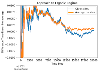
    Figure 1: Two observable's approach to
 ergodicity for Bernoulli Trials. 
Ergodicity appears in many fields, in physics, chemistry and natural sciences but in economics to machine learning as well. Recall that, ergodicity in physics and mathematical definition diverges significantly due to Birkhoff's statistical definition against Boltzmann's physical approach. Here we will follow Birkhoff's definition of ergodicity which is a statistical one. The basic notion of ergodicity is confusing even among experienced  academic circles. The primary misconception is that ergodicity is attributed to a process, a given process being ergodic. We address this by pointing out that ergodicity appears as a regime or a window so to speak for a given process's time-evolution and it can't be attributed to an entire generating process.    

No such thing as ergodic process but ergodic regime given observable

A process being ergodic is not entirely true identification. Ergodicity is a regime over a given time window for a given observable derived from the process. This is the basis of ensemble theory from statistical physics.  Most of the processes generates initially a non-ergodic regime given an observable.  In order to identify an ergodic regime,  we need to define for a discrete setting : 

  1. the ensemble (sample space) : In discrete dynamics we also have an alphabet that ensemble is composed of.
  2. an observable defined over the sample space.
  3. a process (usually dynamics on the sample space evolving over-time).
  4. a measure and threshold to discriminate ergodic to non-ergodic regimes. 
Interesting thing is that different observables on the  same ensemble and the process may generate different ergodic regimes.  

 What are the processes and regime mathematically?

A process is essentially a dynamical system mathematically.  this includes stochastic models and as well as deterministic systems sensitive to initial conditions. Prominently these both combined in Statistical Physics. A regime mathematically implies a range of parameters or a time-window that a system behaves very differently. 

 Identification of ergodic regime
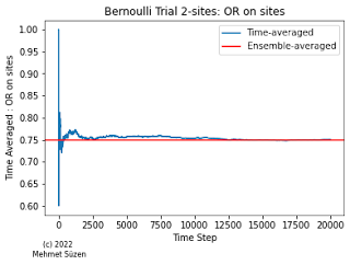
Figure 2: Evolution of
time-averaged OR observable.
The main objective of finding out if dynamics produced by the process on our observable enters or in an ergodic regime is to measure if ensemble-averaged observable is equivalent to time-averaged observable value. Here equivalence is a difficult concept to address quantitatively. The simplest measure would be to check if $\Omega = \langle A \rangle_{ensemble} - \langle A \rangle_{time}$ is close to zero, i.e., vanishing. $ \Omega$ being the ergodicity measure and $A$ is the observable with different averaging procedure. This is the definition we will use here. However, beware that in the physics literature there are more advanced measures to detect ergodicity, such as considering diffusion-like behaviour, meaning that the transition from non-ergodic to ergodic regime is not abrupt but have a diffusing approach to ergodicity.  
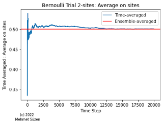
Figure 3: Evolution of
time-averaged mean.

In some other academic fields approach to ergodic regime has different names not strictly but closely related, such as in chemical physics or molecular dynamics, equilibration time, relaxation time, equilibrium, steady-state for a given observable, in statistics Monte Carlo simulations, it is usually called burn out period. Not always, but in ergodic regime, observable is stationary and time-independent. In Physics, this is much easier to distinguish because time-dependence, equilibrium and stationarity are tied to energy transfer to the system. 

Ergodic regime not ergodic process : An example of Bernoulli Trials

Apart from real physical processes such as Ising Model, a basic process we can use to understand how ergodic regime could be detected using Bernoulli Trials. 

Here for a Bernoulli trials/process, we will use random number generators for a binary outcome, i.e., RNG Marsenne-Twister  to generate time evolution of an observables on two sites:  Let's say we have two sites  $x, y \in \{1, 0\}$.  The ensemble of this two site system $xy$ is simply the sample space of all possible outcomes $S=\{10, 11, 01, 00\}$. Time evolution of such two site system is formulated here as choosing $\{0,1\}$  for a given site at a given time, see Appendix Python notebook. 

Now, the most important part of checking ergodic regime is that we need to define an observable over two side trials. We denote two observable as $O_{1}$, which is an OR operation between sites, and $O_{2}$ is averaged over two sites. Since our sample space is small, we can compute the ensemble average observables analytically:

  • $O_{1}  =  (x+y)/2$  then  $10, 11, 01, 00  ;  (1/2 + 2/2 + 1/2 + 0 ) /4 = 0.5$
  • $O_{2}  =  x OR y$ then   $10, 11, 01, 00  ;  ( 1  + 1 + 1 + 0 )/4 = 0.75$   

We can compute the time-averaged observables over time via simulations, but their formulation are know as follows: 

  •  Time average for $O_{1}$ at time $t$  (current step)  is   $ \frac{1}{t} \sum_{i=0}^{t} (x_{i}+y_{i})/2.0$
  • Time average for $O_{2}$ at time $t$  (current step)  is   $ \frac{1}{t} \sum_{i=0}^{t} (x_{i} OR y_{i})$.

One of the possible trajectories are shown in Figure 2 and 3. For approach to ergodicity measure, we shown this at Figure 1. Even though, we should run multiple trajectories to have error estimates, we can clearly see that ergodicity regime starts after 10K steps, at least. Moreover, different observables have different decay rates to ergodic regime.  From preliminary simulation, it appears to be OR observable converges slower, though this is a single trajectory.

Conclusion

We have shown that manifestation of the ergodic regime depends on the time-evolution of the observable given a measure of ergodicity, i.e., a condition how ergodicity is detected. This exposition should clarify that a generating process does not get an attribute of "ergodic process" rather we talk about "ergodic regime" depending on observable and the process over temporal evolution. Interestingly, from Physics point of view, it is perfectly possible that an observable attains ergodic regime and then falls back to non-ergodic regime.

Further reading

Appendix: Code

Bernoulli Trial example we discussed is available as a Python notebook on github here

Please cite as follows:

 @misc{suezen22ergoreg, 
     title = {A misconception in ergodicity: Identify ergodic regime not ergodic process}, 
     howpublished = {\url{http://science-memo.blogspot.com/2022/05/ergodic-regime-not-process.html}, 
     author = {Mehmet Süzen},
     year = {2022}
}  

Wednesday, 28 July 2021

Deep Learning in Mind a Gentle Introduction to Spectral Ergodicity

Preamble

    Figure: Monalisa on
Eigenvector grids (Wikipedia)

In the post, A New Matrix Mathematics for Deep Learning : Random Matrix Theory of Deep Learning, we have outlined a new mathematical concepts that are aimed at deep learning but in general belonging to applied mathematics. Here, we dive into one of the concepts,  spectral ergodicity. We aimed at conveying what does it mean and how to compute spectral ergodicity for a set of matrices, i.e., ensemble. We will use a visual aid and verbal descriptions of steps to produce a quantitative measure of spectral ergodicity. 

The idea of spectral ergodicity comes from quantum statistical physics but it is recently revived for deep learning as a new concept in order to accommodate mathematical needs of explaining and understanding the complexity of deep learning architectures.

Understanding Spectral Ergodicity

The concept of ergodicity can get quiet mathematical even for a professional mathematician.  A practical understanding of ergodicity  could lead to the law of large numbers statistically speaking. However, observed ergodicity for ensemble of matrices, i.e. over their eigenvalue spectrum, are not formally defined before in the literature, and only appeared in statistical quantum mechanics in a specialised case.  Here we do a formal definition gently.

The spectral ergodicity of snapshot of values from $M$ matrices, where they are $N \times N$ sizes,  denoted by $\Omega$, can be produce with the following steps:
  1. Compute eigenvalues of $M$ matrices separately.  
  2. Produce equidistance spectra of matrices out of eigenvalues, i.e., histograms with $b_{k}$ bins. Each cell in the Figure corresponds to bin in the spectra of the matrices. 
  3. Compute average values over each bin across  $M$ matrices.
  4. Computing root mean square deviation that went to each bin from $M$ matrices from corresponding ensemble averaged value and average over $M$ and $N$. This will give a distribution, $\Omega=\Omega(b_{k})$, which represents spectral ergodicity value, think as a snapshot value of a dynamical process.
Attentive reader would notice that normally, measures of ergodicity leads to a single value, such as in spin-glasses, but here we obtain ergodicity as a measure distribution. This stems from the fact that our observable is not univariate but it is a multivariate measure over spectra of the matrix, i.e., bins in the histogram of eigenvalues.  

Why spectral ergodicity important for deep learning? 

The reason why this measure is so important lies in dynamics and consistency in measuring observables (no nothing to do with quantum mechanics but time and ensemble averages classically). Normally we can't measure ensemble averages. In experimental conditions the measurement we do is usually a time averaged value. This is exactly what happens when we train deep neural network, i.e, ergodicity of weight matrices. Essentially, spectral ergodicity would capture deep neural network's characteristics.
Outlook

The way we express spectral ergodicity here would only consider all layer having the same size.  One would need a more advanced computation of spectral ergodicity for more realistic architectures, which is called cascading Periodic Spectral Ergodicity measure suitable as a complexity measure for deep learning.  The computation of such measure is more involved and spectral ergodicity we cover here is the first step.

Cite this post with  Deep Learning in Mind Very Gentle Introduction to Spectral Ergodicity, Mehmet Süzen, (2021) https://science-memo.blogspot.com/2021/07/deep-learning-random-matrix-theory-spectral-ergodicity.html 

Saturday, 14 November 2020

Shannon's Entropy: Why it is called Entropy?


Ludwig Boltzmann
The story (legend) goes like this, von Neumann was asked by Shannon what he thinks and suggested Shannon call it entropy. 

Shannon's entropy is actually a toy version of Boltzmann's entropy. It is a toy version because it only considers configurational entropy of discrete objects without actually describing microstates. The more interesting connection where almost no-one knows is that actually, Birkhoff's ergodic theory has legitimised Shannon's entropy as his version of ergodicity is the toy version of Boltzmann. Well, Gibbs's contribution has a different angle and it is astonishing that why von Neumann omitted that is interesting.                                                                                                      

Shannon's entropy should be called von Neumann-Boltzmann-Shannon Entropy not only Shannon, maybe adding Birkhoff in the team. 


Cite as 

 @misc{suezen20sew, 
     title = {Shannon's Entropy: Why it is called Entropy? }, 
     howpublished = {\url{https://science-memo.blogspot.com/2020/11/shannons-entropy-why-it-is-called.html}, 
     author = {Mehmet Süzen},
     year = {2020}
}  


Postscripts

  • Ergodicity is an intricate subject: Boltzmann's and Birkoff's differing approaches.
  • Jaynes extensively studied the connection, and his interpretation was similar, he said von Neumann-Shannon expression being a " a more primitive concept" and using statistical mechanical ideas to bring in a mathematical tool for statistical inference. See his papers I and II


(c) Copyright 2008-2024 Mehmet Suzen (suzen at acm dot org)

Creative Commons License
This work is licensed under a Creative Commons Attribution 4.0 International License.