Misconceptions on non-temporal learning: When do machine learning models qualify as prediction systems?

Preamble

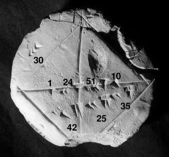
    Babylonian Tablet for 
square root of 2.
 (Wikipedia)

Prediction implies a mechanics, as in knowing a form of a trajectory over time.  Strictly speaking a predictive system implies knowing a solution to the path, set of variable depending on time, time evolution of the system under consideration. Here, we define semi-informally how a prediction system is defined mathematically and show how non-temporal learning can be mapped into a prediction system. 

Temporal learning : Recurrence, trajectory and sequences

A trajectory can be seen as a function of time, identified in recurrence manner. It means $x(t_{i})=f(x_{i-1})$. However, this is one of the possible definitions. The physical equivalent of this appears as a solution to ordinary differential equation, such as the velocity $v(t) = dx(t)/dt$, recurrence on its solution. On the other hand machine learning, an empirical approach is taken and a sequence data such as natural language or a log events occurring in sequence. Any modelling on such data is called temporal learning. This includes classical time-series algorithms, gated units in deep learning and differential equations.

Definition: A prediction system  $\mathscr{F}$ that is build with data $D$ but utilised for a data that is not used in building it $D'$, qualified as such if both $D$ and $D'$ are temporal sets and output of the system is a horizon $\mathbb{H}$, that is a sequence. 

Using non-temporal supervised learning is interpolation or extrapolation

Often practice in industry to turn temporal interactions into flat set of data vectors,  $v_{i}$, $i$ corresponds to a time point or an arbitrary property of the dataset resulting in breaking the temporal associations and causal links.  This could also manifest as set of images with some labels which has no ordering or associational property in the dataset. Even though our system build upon these non-temporal datasets, indeed it constituted a learning systems as interpolation or extrapolation. Their utility in using them for $D'$, strictly speaking does not qualify as prediction systems. 

Mapping with pre-processing

A mapping indeed possible from non-temporal data to a temporal one, if their original form is not in temporal form yet. This is been studied in complexity literature. This requires an algorithm to map flattened data vectors we mentioned into a sequence data. 

Mapping with Causality

A distinct models from causal inference are qualified as predictive systems even if they are trained on non-temporal data, because causality establishes a temporal learning.

Non-temporal modals: Do they still learn?

Even though, we exclude non-temporal model utilisation as non-predictive systems, they still classified as learned models. Because their outputs are generated by a learning procedure. 

Conclusion

Differentiation among temporal and non-temporal learning is provided in associational manner. This results into definition of a prediction system, that excludes non-temporal machine learning models: such as models for unlinked set of vectors, a set of numbers mapped from any data modality. 

Further reading & postscript notes

• Practice causal inference: Conventional supervised learning can't do inference
• Causal inference : Editor's selections from the looper repo.
• Causal models usually are not train but validated or so called discovered.

Constants or integrals of motion: Invariants of a dynamical flow

In this post we will shortly review a concept in dynamical systems namely of invariants of a dynamical flow with a simple derivation using famous Lotka-Volterra system as an example, due to Lotka (1925) and Volterra (1927).

Concept

A dynamical flow associated with an observation vector ${\bf y}(t)$ may have functions, $I({\bf y})$ that are time independent, being $dI/dt=0$. The number of invariants and the length of the observation vector have an effect on overall dynamics.

Lotka-Volterra (LV) System

The LV dynamics explains the behaviour between population of the prey $v$  and population of predators $u$, a case of predator-prey model. We will use a special case of the LV dynamics, remember the dot notation, meaning time derivatives, for predators,
$$ \dot{u}  =  u (v-2) $$
and for prays,
$$ \dot{v}  = v (1-u) $$
Observation vector will consist of $y=(u,v)$.

If we divide these equations, hoping that we can collect $u$ and $v$ in separate terms,

$$
\begin{eqnarray}
\frac{\dot{u}}{\dot{v}}            & = & \frac{u (v-2)}{v(1-u)} \\
\dot{u} v (1-u)                            & = & \dot{v} u (v-2) \\
\dot{u} v (1-u) - \dot{v} u (v-2)  & = & 0 \\
\dot{u} (1-u) - \dot{v} u/v (v -2) & = & 0\\
\dot{u} (1-u)/u - \dot{v}(v-2)/v   & = & 0
\end{eqnarray}
$$

If we integrate both sides over time $dt$,
$$
\begin{eqnarray}
\int \frac{1-u}{u} \frac{du}{dt} dt - \int \frac{v-2}{v} \frac{dv}{dt} dt & = &0 \\
\int \frac{1-u}{u}du - \int \frac{v-2}{v} dv & = &0 \\
\end{eqnarray}
$$

Solution of these indefinite integrals yields to a an invariant of the LV dynamics
$$ d I({\bf y})/dt = ln u - u + 2 ln v - v  $$
We have shown one invariant of the system. This is important to determine the structure of the system, such as volume preserving dynamics, i.e., Hamiltonian Dynamics.

Further Reading

• Geometric Numerical Integration, Ernst Hairer, Christian Lubich, Gerhard Wanner, Springer (2002) 
• Arnold, V. I. and A. Avez (1968). Ergodic Problems of Classical Mechanics. New York, Benjamin.

Is ergodicity a reasonable hypothesis? Understanding Boltzmann's ergodic hypothesis

Ergodic vs. non-ergodic
trajectories (Wikipedia)

Many undergraduate Physics students barely study Ergodic Hypothesis in detail. It is usually manifested as ensemble averages being equal to time averages. While the concept of the statistical ensemble maybe accessible to students, when it comes to ergodic theory and theorems,  where higher level mathematical jargon kicks in, it maybe confusing for the novice reader or even practicing Physicists and educator what does ergodicity really mean. For example recent pre-print titled "Is ergodicity a reasonable hypothesis?" defines the ergodicity as follows:

...In the physics literature "ergodicity" is taken to mean that a system, including a macroscopic one, visits all microscopic states in a relatively short time...[link]

Visiting all microscopic states is not a pre-condition for ergodicity from statistical physics stand point. This form of the theory is the manifestation of strong ergodic hypothesis because of the Birkhoff theorem and may not reflect the physical meaning of ergodicity.  However,  the originator of ergodic hypothesis,  Boltzmann, had a different thing in mind in explaining how a system approaches to thermodynamic equilibrium. One of the best explanations are given in the book of J. R. Dorfman, titled An introduction to Chaos and Nonequilibrium Statistical Mechanics [link], in section 1.3, Dorfman explains what Boltzmann had in mind:

...Boltzmann then made the hypothesis that a mechanical system's trajectory in phase-space will spend equal times in regions of equal phase-space measure. If this is true, then any dynamical system will spend most of its time in phase-space region where the values of the interesting macroscopic properties are extremely close to the equilibrium values...[link]

Saying this, Boltzmann did not suggest that a system should visit ALL microscopic states.  His argument only suggests that only states which are close the equilibrium has more likelihood to be visited.

Postscript (June 2022)

The sufficiency of Sparse Visits: Physical states are rarely fine-grained

A requirement for attaining ergodicity is visiting all possible states or regions due to the ergodic theorems of Birkhoff and von Neumann. This requirement is not correct for Physics. The key concepts here are coarse-graining and the sufficiency of sparse visits. Most of the physical systems have equally likely states.

The generated dynamics would rarely need to visit all accessible states or regions. Physical systems are rarely fine-grained and have a degree of sparseness, reducing their astronomically large number of states to a handful. In summary, visiting all physical states or regions in time averages is not strictly needed for the physics definition of ergodicity.

A collection of regions or multiple states with a higher probability will need to be covered to achieve thermodynamic equilibrium. A concept of “sufficiency of sparse visits”. This approach makes physical experiments possible over a finite time consistent with thermodynamics.