Showing posts with label representation learning. Show all posts

Saturday, 28 January 2023

Misconceptions on non-temporal learning: When do machine learning models qualify as prediction systems?

Preamble

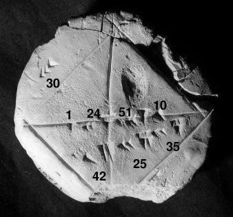
    Babylonian Tablet for 
square root of 2.
 (Wikipedia)
Prediction implies a mechanics, as in knowing a form of a trajectory over time.  Strictly speaking a predictive system implies knowing a solution to the path, set of variable depending on time, time evolution of the system under consideration. Here, we define semi-informally how a prediction system is defined mathematically and show how non-temporal learning can be mapped into a prediction system. 

Temporal learning : Recurrence, trajectory and sequences

A trajectory can be seen as a function of time, identified in recurrence manner. It means $x(t_{i})=f(x_{i-1})$. However, this is one of the possible definitions. The physical equivalent of this appears as a solution to ordinary differential equation, such as the velocity $v(t) = dx(t)/dt$, recurrence on its solution. On the other hand machine learning, an empirical approach is taken and a sequence data such as natural language or a log events occurring in sequence. Any modelling on such data is called temporal learning. This includes classical time-series algorithms, gated units in deep learning and differential equations.

Definition: A prediction system  $\mathscr{F}$ that is build with data $D$ but utilised for a data that is not used in building it $D'$, qualified as such if both $D$ and $D'$ are temporal sets and output of the system is a horizon $\mathbb{H}$, that is a sequence. 

Using non-temporal supervised learning is interpolation or extrapolation

Often practice in industry to turn temporal interactions into flat set of data vectors,  $v_{i}$, $i$ corresponds to a time point or an arbitrary property of the dataset resulting in breaking the temporal associations and causal links.  This could also manifest as set of images with some labels which has no ordering or associational property in the dataset. Even though our system build upon these non-temporal datasets, indeed it constituted a learning systems as interpolation or extrapolation. Their utility in using them for $D'$, strictly speaking does not qualify as prediction systems. 

Mapping with pre-processing

A mapping indeed possible from non-temporal data to a temporal one, if their original form is not in temporal form yet. This is been studied in complexity literature. This requires an algorithm to map flattened data vectors we mentioned into a sequence data. 

Mapping with Causality

A distinct models from causal inference are qualified as predictive systems even if they are trained on non-temporal data, because causality establishes a temporal learning.

Non-temporal modals: Do they still learn?

Even though, we exclude non-temporal model utilisation as non-predictive systems, they still classified as learned models. Because their outputs are generated by a learning procedure. 

Conclusion

Differentiation among temporal and non-temporal learning is provided in associational manner. This results into definition of a prediction system, that excludes non-temporal machine learning models: such as models for unlinked set of vectors, a set of numbers mapped from any data modality. 

Further reading & postscript notes


Monday, 20 June 2022

Empirical risk minimization is not learning :
A mathematical definition of learning and re-understanding of overfitting and Occam's razor in machine learning

    Simionescu Function (Wikipedia)

Preamble

The holy grail of machine learning appears to be the empirical risk minimisation. However, on the contrary to general dogma,  the primary objective of machine learning is not risk minimisation per se but mimicking human or animal learning. Empirical risk minimisation is just a snap-shot in this direction and is part of a learning measure, not the primary objective.

Unfortunately, all current major machine learning libraries are implementing empirical risk minimisation as primary objective, so called a training, manifest as usually .fit. Here we provide a mathematical definition of learning in the language of empirical risk minimisation and its implications on two very important concepts, overfitting and Occam's razor.

Our exposition is still informal but it should be readable for experienced practitioners.

Definition: Empirical Risk Minimization

Given set of $k$ observation $\mathscr{O} = \{o_{1}, ..., o_{k} \}$ where $o_{i} \in \mathbb{R}^{n}$, $n$-dimensional vectors.  Corresponding labels or binary classes, the set $\mathscr{S} = \{ s_{1}, .., s_{k}\}$, with $s_{i} \in \{0,1\}$ is defined. A function $g$  maps observations to classes $g: \mathscr{O} \to \mathscr{S}$.  An error function (or loss) $E$ measures the error made by the estimated map function $\hat{g}$ compare to true map function $g$,  $E=E(\hat{g}, g)$.  The entire idea of supervised machine learning boils down to minimising a functional called ER (Empirical Risk), here we denoted by $G$, it is a functional, meaning is a function of function, over the domain $\mathscr{D} = Tr(\mathscr{O} x \mathscr{S})$ in discrete form, $$ G[E] = \frac{1}{k} {\Large \Sigma}_{\mathscr{D} }  E(\hat{g}, g) $$.  This is so called a training a machine learning model, or an estimation for  $\hat{g}$. However, testing this estimate on the new data is not the main purpose of the learning.

Definition: Learning measure 

A learning measures $M$, on $\hat{g}$ is defined over set of $l$ observations with increasing size, $\Theta = \{ \mathscr{O}_{1}, ..., \mathscr{O}_{l}\}$ whereby size of each set is monotonically higher, meaning that $ | \mathscr{O}_{1}| < | \mathscr{O}_{2}| , ...,< | \mathscr{O}_{l}|$.

Definition: Empirical Risk Minimization with a learning measure (ERL)

Now, we are in a position to reformulate ER with learning measure, we call this ERL. This come with a testing procedure.

If empirical risks $G[E_{j}]$ lowers monotonically, $ G[E_{1}] > G[E_{2}] > ... > G[E_{l}]$, then we said the functional form of $\hat{g}$ is a learning over the set  $\Theta$.  

Functional form of $\hat{g}$ : Inductive bias

The functional form implies a model selection, and a technical term of this also known as inductive bias with other assumptions, meaning the selection of complexity of the model, for example a linear regression or nonlinear regression.

Re-understanding of overfitting and Occam's razor from ERL perspective 

If we have two different ERLs on $\hat{g}^{1}$ and $\hat{g}^{2}$. Then overfitting is a comparison problem between monotonically increasing empirical risks. If model, here an inductive bias or a functional form, over learning measure, we select the one with "higher monotonicity" and the less complex one and call the other overfitted model. Complexity here boils down to functional complexity of $\hat{g}^{1}$ and  $\hat{g}^{2}$  and overfitting can only be tested with two models over monotonicity (increasing) of ERLs.

Conclusions

In the age of deep learning systems, the classical learning theory needs an update on how do we define what is learning beyond a single shot fitting exercise. A first step in this direction would be to improve upon basic definitions of Empirical Risk (ER) minimisation that would reflect real-life learning systems similar to forgetting mechanism proposed by Ebbinghaus. This is consistent with Tom Mitchell's definition of operational machine learning. A next level would be to add causality in the definition.

Please cite as follows:

 @misc{suezen22erm, 
     title = { Empirical risk minimization is not learning : A mathematical definition of learning and re-understanding of overfitting and Occam's razor in machine learning}, 
     howpublished = {\url{http://science-memo.blogspot.com/2022/06/empirical-risk-minimisation-learning-curve.html}}, 
     author = {Mehmet Süzen},
     year = {2022}

}  

Postscript Notes

Following notes are added after initial release 

Postscript 1: Understanding overfitting as comparison of inductive biases

ERM could be confusing for even experienced researchers. It is indeed about risk measure. We measure the risk of a model, i.e., machine learning procedure that how much error would it make on the  given new data distribution, as in risk of investing. This is quite a similar notion as in financial risk of loss but not explicitly stated. 


Moreover, a primary objective of machine learning is not ERM but measure learning curves and pair-wise comparison of  inductive biases, avoiding overfitting.  An inductive bias, here we restrict the concept as in model  type,  is a model selection step: different  parametrisation of the same model are still the same inductive bias.  That’s why standard training-error learning curves can’t be used to detect overfitting alone. 

Postscript 2: Learning is not to optimise: Thermodynamic limit, true risk and accessible learning space

True risk minimisation in machine learning is not possible, instead we rely on ERM, i.e., Emprical Risk Minimisation.  However, the purpose of machine learning algorithm is not to minimise risk, as we only have a  partial knowledge about the reality through data.  Learning implies finding out a region  in accessible learning space whereby there is a monotonic increase in the objective; ERM is only a single point on this space, the concept rooted in German scientist Hermann Ebbinghaus  work on memory.


There is an intimate connection to thermodynamic limit and true risk in this direction as an open research.  However, it doesn’t imply infinite limit of data, but the observable’s behaviour. That’s why full empiricist approaches usually requires a complement of a physical laws,  such as Physics Informed Neural Networks (PINNs) or Structural Causal Model (SCM).

Postscript 3: Missing abstraction in modern machine learning libraries 

Interestingly current modern machine learning libraries stop abstracting further than fitting: .fit and .predict. This is short of learning as in machine learning. Learning manifest itself In learning curves. .learn functionality can be leveraged beyond fitting and if we are learning via monotonically increasing performance. Origin of this lack of tools for .learn appears to be how Empirical Risk Minimisation (ERM) is formulated on a single task.
Sunday, 27 December 2020

Statistical Physics Origins of Connectionist Learning:
Cooperative Phenomenon to Ising-Lenz Architectures

This is an informal essay in aiming at raising awareness that Statistical Physics played a foundational role in deep learning and neural networks in general beyond being a mare analogy but its origin

Article version of this post is available here: doi. and on HAL Open Science

Preamble

A short account of origins of mathematical formalism of neural networks is presented for physicists and computer scientist in basic discrete mathematical setting informally. The discourse of the development of mathematical formalism on the dynamics of lattice models in statistical physics and learning internal representations of neural networks as discrete architectures as quantitative tools evolve in two almost distinct fields more than half a century with limited overlap. We aim at bridging the gap by claiming that the analogy between two approaches are not artificial but naturally occuring due to how modelling cooperative phenomenon is constructed. We define the Lenz-Ising architectures (ILAs) for this purpose.

Introduction


Tartan Ising Model
Figure: Tartan Ising Model
(Linas Viptas-Wikipedia)
Understanding natural or artificial phenomenon in the language of discrete mathematics is probably one of the most powerful toolbox scientist use [1]. Large portion of computer science and statistical physics deals with such finite structures. One of the most prominent successful usage of such approach was Lenz and Ising’s work on modelling ferromagnetic materials [2–5] and neural networks as a model to biological neuronal structures [6–8].

The analogy between two areas of distinct research have been pointed out by many researchers [9–13]. However, the discourse and evolution of these approaches were kept as two distinct research fields and many innovative approaches rediscovered under different names.

Cooperative Phenomenon

Statistical definition of cooperative phenomenon pioneered by Wannier and Kremer [14–16]. Even though their technical work focused on extension of Ising model to 2D with cyclic boundary condition and introduction of exact solutions with matrix algebra, they were the first to document the potential of how Lenz-Ising model actually represent a more generic system than merely model to ferromagnets, namely anything falls under cooperative phenomenon can be addressed with Lenz-Ising type model, summarised in Definition 1.

Definition 1: Cooperative phenomenon of Wannier type  [14]: Set of $N$ discrete units, $\mathscr{U}$, identified with a function $s_{i}$, i=1,..,N forms a collection or assembly. The function that identifies the units is a mapping $s_{i}: \mathbb{R} \rightarrow \mathbb{R}$. A statistic $\mathscr{S}$ applied on $\mathscr{U}$ is called cooperative phenomenon of Wannier type $\mathscr{W}$.

A statistic $\mathscr{S}$ can be any mapping or set of operations on the assembly of units $\mathscr{U}$ . For example inducing ordering on the assembly of units and summation over  $s_{i}$ values, would corresponds to non-interacting magnetic system with unit external field or non-connected set of neurons capacity of inhibition or exhibition. However, amazingly, Definition 1 is so generic that Rosenblatt’s perceptron [17], current deep learning systems [18] and complex networks [19] falls into this category as well. 

The originality of Cooperative phenomenon of Wannier type comes on a secondary concept, so called event propagation as given in Definition 2.

Definition 2. Event propagation [14] An event is defined as a snapshot of cooperative phenomenon of Wannier type $\mathscr{W}$. If an event takes place of one unit of assembly $\mathscr{U}$, the same event will be favored by other units, this is expressed as event propagation between two disjoint set of units $\mathscr{E}(u_{1}, u_{2})$, and $u_{1} \cap u_{2} = \varnothing$ and $u_{1}, u_{2} \in \mathscr{U}$ and with an additional statistic $\mathscr{S}$ is defined.

The parallels between Wannier’s event propagations are remarkably the same as of neural network formalism defined by McCulloch-Pitts-Kleene [6,7], not only conceptually but matematical treatment is identical and originates from Lenz-Ising model’s treatment of discrete units. As we mentioned, this goes beyond doubt not a simple analogy but forms a generic framework as envisioned by Wannier. The similarity between ferromagnetic systems and neural networks is probably first documented directly by Little [8]: Spin states of magnetic spins corresponds to firing state of a neuron. Unfortunately, Little only see it as simple analogy, and missed the opportunity provided by Wannier as a generic natural phenomenon of cooperation.

The conceptual similarity and inference on Wannier’s event propagation appears to be quite close to Hebb’s learning [20] and gives natural justification for backpropagation for multilayered networks. History of backpropagation is exhaustively studied elsewhere [18].

Lenz-Ising Architectures (ILAs): Ferromagnets to Nerve Nets


Ernst Ising
 Image owner APS - Physics Today :
Obituary
As we established two basic definitions of cooperative phenomenon, we can now define a generic setting of Lenz-Ising model that captures both physics literature that extensively used this in so called spin-glasses research and for neural networks. A guiding principle will be based on Wannier’s definition of cooperative phenomenon.

Definition: Lenz-Ising Architectures (ILAs) 
Given Wannier type cooperative phenomenon $\mathscr{W}$, imposing constrains on the discrete units, $\mathscr{U}^{c}$ that they should be spatially correlated on the edges $E$ of an arbitrary graph $\mathscr{G}(E, V)$ with ordering and with vertices $V$ of the arbitrary graph carring coupling weight between connected two units with biases. Set of event propagations $\mathscr{E}^{c}$ defined on the cooperative phenomeon can induce dynamics on defining vertice weights, or vice versa. ILAs are defined as statistic $\mathscr{S}$ applied to $\mathscr{U}^{c}$ with propagations $\mathscr{E}^{c}$. 

Lenz-Ising Architectures (ILAs) should not be confused with graph neural networks as it does not model data structures. It could be seen as subset of graph dynamical systems in some sense but formal connections should be established elsewhere. However, primary characteristic of ILAs are that it is conceptual and mathematical representation of spin-glass systems (including Lenz-Ising, Anderson, Sherrington-Kirkpatrick, Potts systems) and neural networks (including recurrent and convolutional networks) under the same umbrella.

 Learning representations inherent in Metropolis-Glauber dynamics

The primary originality in any neural network research papers lies in so called learning representation from data and generalisation. However, it isn’t obvious to the that community that actually spin-glasses are capable of learning representations inherently by induced dynamics such as Metropolis or Glauber dynamics by construction, as an inverse problem.

In physics literature this appears as finding a solution to the problem of how to express free energy and minimisation of this with respect to weights or coupling coefficients, This is noting but a learning represenations. Usually a simulation approach is taken as a route, for example Monte Carlo techniques [5, 21, 22] via Metropolis or Glauber dynamics. The intimate connection between concepts of ergodicity and learning in deep learning is recently shown [13,23,24] in this context.

Roy J. Glauber (Wikipedia)  
Glauber dynamics

As we argued earlier the generic definition provided by Wannier on cooperative phenomenon and ILAs; there is an intimate connection with learning and so called solving spin-glasses that usually boils down to computing free energies as mentioned. And a link between two distinct fields, computing backpropagation and free energies are natural candidates to establish equivalence relations.

Conclusions and Outlook

Apart from honouring physicists Lenz and Ising, based on understanding of cooperative phenomenon’s origins, naming the research outpus from of spin-glasses and neural networks under an umbrella term Lenz-Ising architectures (ILAs) is historically accurate and technically a resonable naming scheme under the overwhelming evidence given in the literature. This is akin to naming current computers with von Neumann architectures. This forms the origins of connectionist learning from statistical physics, where this approach currently enjoying vast engineering success today.

The rich connection between two areas in computer science and statistical physics should be celebrated. For more fruitful collaborations, both literatures, embracing large statistics literature as well, should converge much more closely. This would help communities to avoid awkward situations of reinventing the wheel again and hindering recognition of the work done by physicists decades earlies, i.e., Ising and Lenz.

 Notes

No competing or other kind of conflict of interest exists. This work is produced solely with the aim of scholarly work and does not have any personal nature at all. This essay is dedicated in memory of Ernst Ising for his contribution to physics of ferromagnetic materials, now seems to have far more implications.

References

[1] Kenneth H Rosen. Handbook of Discrete and Combinatorial Mathematics. CRC Press, 1999. 

[2] W.Lenz. Beitrag zum Verstl ̈andnis der Magnetischen Erscheinungen in Festen Korpern. Phys.Z21:613, 1920.

[3] Ernst Ising. Beitrag zur Theorie des Ferromagnetismus. Zeitschrift furr Physik, 31(1):253–258, 1925.

[4] Thomas Ising, Reinhard Folk, Ralph Kenna, Bertrand Berche, and Yurij Holovatch. The fate of Ernst Ising and the fate of his model. arXiv preprint arXiv:1706.01764, 2017.

[5] David P Landau and Kurt Binder. A guide to Monte Carlo Simulations in Statistical Physics. Cambridge University Press, 2014.

[6] W.S. McCulloch and W.H. Pitts. A Logical Calculus of the Ideas Imminent in Nervous Activity.Bull. Math. Biophys.,(5), pages 115–133.

[7] Stephen Cole Kleene. Representation of Events in Nerve Nets and Finite Automata. Technical report, RAND Project, Santa Monica, 1951.

[8] W. A. Little. The Existence of Persistent States in the Brain. Mathematical Biosciences, 19(1-2):101–120, 1974.

[9] P Peretto. Collective Properties of Neural Networks: a Statistical Physics Approach. Biological Cybernetics, 50(1):51–62, 1984.

[10] Jan L van Hemmen. Spin-glass Models of a Neural Network. Physical Review A, 34(4):3435, 1986.

[11] Haim Sompolinsky. Statistical Mechanics of Neural Networks. Physics Today, 41(21):70–80,1988.

[12] David Sherrington. Neural Networks: the Spin Glass Approach. In North-Holland MathematicalLibrary, volume 51, pages 261–291. Elsevier, 1993.

[13] Yasaman Bahri, Jonathan Kadmon, Jeffrey Pennington, Sam S Schoenholz, Jascha Sohl-Dickstein, and Surya Ganguli. Statistical Mechanics of Deep Learning. Annual Review of Condensed Matter Physics, 2020.

[14] Gregory H Wannier. The Statistical Problem in Cooperative Phenomena. Reviews of Modern Physics, 17(1):50, 1945.

[15] Hendrik A Kramers and Gregory H Wannier. Statistics of the two-dimensional ferromagnet.Part I. Physical Review, 60(3):252, 1941.

[16] Hendrik A Kramers and Gregory H Wannier. Statistics of the two-dimensional ferromagnet.Part II. Physical Review, 60(3):263, 1941.

[17] C van der Malsburg. Frank Rosenblatt: principles of neurodynamics: perceptrons and the theory of brain mechanisms. In Brain theory, pages 245–248. Springer, 1986.

[18] J. Schmidhuber. Deep learning in Neural Networks: An overview. Neural networks, 61:85–117, 2015. & Yoshua Bengio, Yann Lecun, Geoffrey Hinton, Communications of the ACM, July 2021, Vol. 64 No. 7, Pages 58-65 (2021) link

[19] Duncan J Watts and Steven H Strogatz. Collective dynamics of ‘small-world’networks. Nature,393(6684):440, 1998.

[20] Donald Olding Hebb. The Organization of Behavior: a Neuropsychological Theory. J. Wiley;Chapman & Hall, 1949.

[21] Mehmet Suezen. Effective ergodicity in single-spin-flip dynamics. Physical Review E, 90(3):032141, 2014.

[22] Mehmet Suezen. Anomalous diffusion in convergence to effective ergodicity. arXiv preprint arXiv:1606.08693, 2016.

[23] Mehmet Suezen, Cornelius Weber, and Joan J Cerda. Spectral ergodicity in deep learning architectures via surrogate random matrices. arXiv preprint arXiv:1704.08303, 2017.

[24] Mehmet Suezen, JJ Cerda, and Cornelius Weber. Periodic Spectral Ergodicity: A Complexity Measure for Deep Neural Networks and Neural Architecture Search. arXiv preprint arXiv:1911.07831, 2019.


Postscript 1:

(Deep) Machine learning as a subfield of statistical physics

Often researchers considers some machine learning methods
under different umbrella terms compare to established
statistical physics. However, beyond being mare analogy,  
application of these methods are quite striking. Consequently,
there is a great tradition in machine learning practice 
of being sub-field of statistical physics with explicit
classification within PACS. 

Hopfield Networks <- Ising-Lenz model
Boltzmann Machines <- Sherrington-Kirkpatrick model
Diffusion Models <- Langevin Dynamics, Fokker-Planck Dynamics
Softmax <- Boltzmann-Gibbs connection to partition function 
Energy Based Models <- Spin-glasses, Hamiltonian dynamics

For this reason, we provide semi-formal mathematical definitions
in the recent article, establishing that deep learning architectures 
should be called Ising-Lenz Architectures (ILAs), akin to calling 
current computers having von Neumann architectures.

(c) Copyright 2008-2024 Mehmet Suzen (suzen at acm dot org)

Creative Commons License
This work is licensed under a Creative Commons Attribution 4.0 International License.