Tuesday, 20 September 2022

Building robust AI systems: Is an artificial intelligent agent just a probabilistic boolean function?


Preamble
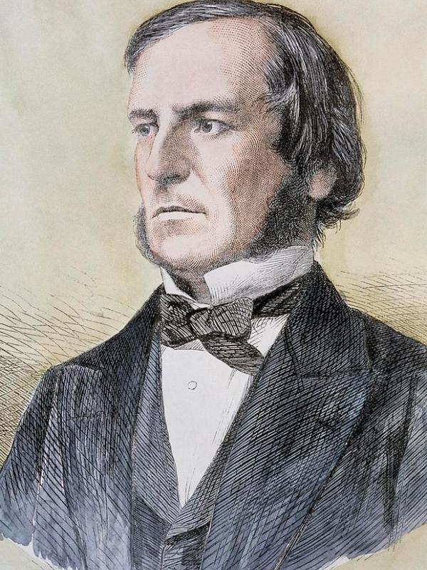
    George Boole (Wikipedia)

Agent, AI agent or an intelligent agent is used often to describe algorithms or AI systems that are released by research teams recently. However, the definition of an intelligent agent (IA) is a bit opaque. Naïvely thinking, it is nothing more than a decision maker that shows some intelligent behaviour. However, making a decision intelligently is hard to quantify computationally, and probably IA for us is something that can be representable as a Turing machine.  Here, we argue that an intelligent agent in the current AI systems should be seen as a function without side effects outputting a boolean output and shouldn't be extrapolated or compare to human level intelligence.  Causal inference capabilities should be seen as a scientific guidance to this function decompositions without side-effects,  i.e., Human in-the loop Probabilistic Boolean Functions (PBFs).

Computational learning theories are based on binary learners

Two of the major  theories of statistical learning PAC and VC dimensions build upon on "binary learning".  

PAC stands for Probably Approximately Correct, It sets basic framework and mathematical building blocks for defining a machine learning problem from complexity theory. Probably correct implies finding a weak learning function given binary instance set $X=\{1,0\}^{n}$. The binary set or its subsets mathematically called concepts and under certain mathematical conditions a system said to be PAC learnable. There are equivalences to VC and other computation learning frameworks. 

Robust AI systems: Deep reinforcement learning and  PAC

Even though the theory of learning on deep (reinforcement) learning is not established and active area of research. There is an intimate connection with composition of concepts, i.e., binary instance subsets as almost all operations within  deep RL can be viewed as probabilistic Boolean functions (PBFs). 

Conclusion 

Current research and practice in robust AI systems could focus on producing learnable probabilistic boolean functions (PBFs) as intelligent agents, rather than being a human level intelligent agents. This modest purpose might bring more practical fruit than long-term aims of replacing human intelligence. Moreover, theory of computation for deep learning and causality could benefit from this approach. 

Further reading


Tuesday, 5 July 2022

Bayesian rabbit holes: Decoding conditional probability with non-commutative algebra

Preamble

    The White Rabbit
(Wikipedia)

A novice analyst or even experienced (data) scientist would have thought that the bar notation $|$ in representing conditional probability carries some different operational mathematics. Primarily when written in explicit distribution functions $p(x|y)$. Similar approach applies to joint probabilities such as $p(x, y)$ too. One could see a mixture of these, such as $p(x, y | z)$. In this short exposition, we clarify that none of these identifications within arguments of probability do have any different resulting operational meaning. 

Arguments in probabilities: Boolean statement and filtering 

Arguments in any probability are mathematical statements of discrete mathematics that correspond to events in the experimental setting. These are statements declaring some facts with a boolean outcome. These statements are queries to a data set. Such as, if the temperature is above $30$ degrees, $T > 30$. Temperature $T$ is a random variable. Unfortunately, the term random variable is often used differently in many textbooks. It is defined as a mapping rather than as a single variable. The bar $|$ in conditional probability $p(x|y)$, implies statement $x$ given that statement $y$ has already occurred, i.e., if. This interpretation implies that $y$ first occurred before $x$, but it doesn't imply that they are causally linked. The condition plays a role in filtering, a where clause in query languages. $p(x|y)$ boils down to $p_{y}(x)$, where the first statement $y$ is applied to the dataset before computing the probability on the remaining statement $x$.

In the case of joint probabilities $p(x, y)$, events co-occur, i.e., AND statement. In summary, anything in the argument of $p$ is written as a mathematical statement. In the case of assigning a distribution or a functional form to $p$, there is no particular role for conditionals or joints; the modelling approach sets an appropriate structure.

Conditioning does not imply casual direction: do-Calculus do

A filtering interpretation of conditional $p(x|y)$ does not imply causal direction, but $do$ operator does, $p(x|do(y))$. 

Non-commutative algebra: When frequentist are equivalent to Bayesian

Most of the simple filtering operations would result in identical results if reversed. $p(x|y) = p(y|x)$, prior being equal to posterior. This remark implies we can't apply Bayesian learning with commutative statements. We need non-commutative statements; as a result, one can do Bayesian learning with the newly arriving data, i.e., the arrival of new subjective evidence. The reason seems to be due to the frequentist nature of filtering.

Outlook 

Even though we provided some revelations on decoding the operational meaning of conditional probabilities, we suggested that any conditional, joint or any combination of these within the argument of probabilities has no operational purpose other than pre-processing steps. However, the philosophical and practical implications of probabilistic reasoning are always counterintuitive. Probabilistic reasoning is a complex problem computationally. From a causal inference perspective, we are better equipped to tackle these issues with do-Bayesian analysis.  

Further reading

Please Cite as:

 @misc{suezen22brh, 
     title = {Bayesian rabbit holes: Decoding conditional probability with non-commutative algebra}, 
     howpublished = {\url{https://science-memo.blogspot.com/2022/07/bayesian-conditional-noncommutative.html}}, 
     author = {Mehmet Süzen},
     year = {2022}
}  

Monday, 20 June 2022

Empirical risk minimization is not learning :
A mathematical definition of learning and re-understanding of overfitting and Occam's razor in machine learning

    Simionescu Function (Wikipedia)

Preamble

The holy grail of machine learning appears to be the empirical risk minimisation. However, on the contrary to general dogma,  the primary objective of machine learning is not risk minimisation per se but mimicking human or animal learning. Empirical risk minimisation is just a snap-shot in this direction and is part of a learning measure, not the primary objective.

Unfortunately, all current major machine learning libraries are implementing empirical risk minimisation as primary objective, so called a training, manifest as usually .fit. Here we provide a mathematical definition of learning in the language of empirical risk minimisation and its implications on two very important concepts, overfitting and Occam's razor.

Our exposition is still informal but it should be readable for experienced practitioners.

Definition: Empirical Risk Minimization

Given set of $k$ observation $\mathscr{O} = \{o_{1}, ..., o_{k} \}$ where $o_{i} \in \mathbb{R}^{n}$, $n$-dimensional vectors.  Corresponding labels or binary classes, the set $\mathscr{S} = \{ s_{1}, .., s_{k}\}$, with $s_{i} \in \{0,1\}$ is defined. A function $g$  maps observations to classes $g: \mathscr{O} \to \mathscr{S}$.  An error function (or loss) $E$ measures the error made by the estimated map function $\hat{g}$ compare to true map function $g$,  $E=E(\hat{g}, g)$.  The entire idea of supervised machine learning boils down to minimising a functional called ER (Empirical Risk), here we denoted by $G$, it is a functional, meaning is a function of function, over the domain $\mathscr{D} = Tr(\mathscr{O} x \mathscr{S})$ in discrete form, $$ G[E] = \frac{1}{k} {\Large \Sigma}_{\mathscr{D} }  E(\hat{g}, g) $$.  This is so called a training a machine learning model, or an estimation for  $\hat{g}$. However, testing this estimate on the new data is not the main purpose of the learning.

Definition: Learning measure 

A learning measures $M$, on $\hat{g}$ is defined over set of $l$ observations with increasing size, $\Theta = \{ \mathscr{O}_{1}, ..., \mathscr{O}_{l}\}$ whereby size of each set is monotonically higher, meaning that $ | \mathscr{O}_{1}| < | \mathscr{O}_{2}| , ...,< | \mathscr{O}_{l}|$.

Definition: Empirical Risk Minimization with a learning measure (ERL)

Now, we are in a position to reformulate ER with learning measure, we call this ERL. This come with a testing procedure.

If empirical risks $G[E_{j}]$ lowers monotonically, $ G[E_{1}] > G[E_{2}] > ... > G[E_{l}]$, then we said the functional form of $\hat{g}$ is a learning over the set  $\Theta$.  

Functional form of $\hat{g}$ : Inductive bias

The functional form implies a model selection, and a technical term of this also known as inductive bias with other assumptions, meaning the selection of complexity of the model, for example a linear regression or nonlinear regression.

Re-understanding of overfitting and Occam's razor from ERL perspective 

If we have two different ERLs on $\hat{g}^{1}$ and $\hat{g}^{2}$. Then overfitting is a comparison problem between monotonically increasing empirical risks. If model, here an inductive bias or a functional form, over learning measure, we select the one with "higher monotonicity" and the less complex one and call the other overfitted model. Complexity here boils down to functional complexity of $\hat{g}^{1}$ and  $\hat{g}^{2}$  and overfitting can only be tested with two models over monotonicity (increasing) of ERLs.

Conclusions

In the age of deep learning systems, the classical learning theory needs an update on how do we define what is learning beyond a single shot fitting exercise. A first step in this direction would be to improve upon basic definitions of Empirical Risk (ER) minimisation that would reflect real-life learning systems similar to forgetting mechanism proposed by Ebbinghaus. This is consistent with Tom Mitchell's definition of operational machine learning. A next level would be to add causality in the definition.

Please cite as follows:

 @misc{suezen22erm, 
     title = { Empirical risk minimization is not learning : A mathematical definition of learning and re-understanding of overfitting and Occam's razor in machine learning}, 
     howpublished = {\url{http://science-memo.blogspot.com/2022/06/empirical-risk-minimisation-learning-curve.html}}, 
     author = {Mehmet Süzen},
     year = {2022}

}  

Postscript Notes

Following notes are added after initial release 

Postscript 1: Understanding overfitting as comparison of inductive biases

ERM could be confusing for even experienced researchers. It is indeed about risk measure. We measure the risk of a model, i.e., machine learning procedure that how much error would it make on the  given new data distribution, as in risk of investing. This is quite a similar notion as in financial risk of loss but not explicitly stated. 


Moreover, a primary objective of machine learning is not ERM but measure learning curves and pair-wise comparison of  inductive biases, avoiding overfitting.  An inductive bias, here we restrict the concept as in model  type,  is a model selection step: different  parametrisation of the same model are still the same inductive bias.  That’s why standard training-error learning curves can’t be used to detect overfitting alone. 

Postscript 2: Learning is not to optimise: Thermodynamic limit, true risk and accessible learning space

True risk minimisation in machine learning is not possible, instead we rely on ERM, i.e., Emprical Risk Minimisation.  However, the purpose of machine learning algorithm is not to minimise risk, as we only have a  partial knowledge about the reality through data.  Learning implies finding out a region  in accessible learning space whereby there is a monotonic increase in the objective; ERM is only a single point on this space, the concept rooted in German scientist Hermann Ebbinghaus  work on memory.


There is an intimate connection to thermodynamic limit and true risk in this direction as an open research.  However, it doesn’t imply infinite limit of data, but the observable’s behaviour. That’s why full empiricist approaches usually requires a complement of a physical laws,  such as Physics Informed Neural Networks (PINNs) or Structural Causal Model (SCM).

Postscript 3: Missing abstraction in modern machine learning libraries 

Interestingly current modern machine learning libraries stop abstracting further than fitting: .fit and .predict. This is short of learning as in machine learning. Learning manifest itself In learning curves. .learn functionality can be leveraged beyond fitting and if we are learning via monotonically increasing performance. Origin of this lack of tools for .learn appears to be how Empirical Risk Minimisation (ERM) is formulated on a single task.
Wednesday, 11 May 2022

A misconception in ergodicity: Identify ergodic regime not ergodic process

Preamble 

    Figure 1: Two observable's approach to
 ergodicity for Bernoulli Trials. 
Ergodicity appears in many fields, in physics, chemistry and natural sciences but in economics to machine learning as well. Recall that, ergodicity in physics and mathematical definition diverges significantly due to Birkhoff's statistical definition against Boltzmann's physical approach. Here we will follow Birkhoff's definition of ergodicity which is a statistical one. The basic notion of ergodicity is confusing even among experienced  academic circles. The primary misconception is that ergodicity is attributed to a process, a given process being ergodic. We address this by pointing out that ergodicity appears as a regime or a window so to speak for a given process's time-evolution and it can't be attributed to an entire generating process.    

No such thing as ergodic process but ergodic regime given observable

A process being ergodic is not entirely true identification. Ergodicity is a regime over a given time window for a given observable derived from the process. This is the basis of ensemble theory from statistical physics.  Most of the processes generates initially a non-ergodic regime given an observable.  In order to identify an ergodic regime,  we need to define for a discrete setting : 

  1. the ensemble (sample space) : In discrete dynamics we also have an alphabet that ensemble is composed of.
  2. an observable defined over the sample space.
  3. a process (usually dynamics on the sample space evolving over-time).
  4. a measure and threshold to discriminate ergodic to non-ergodic regimes. 
Interesting thing is that different observables on the  same ensemble and the process may generate different ergodic regimes.  

 What are the processes and regime mathematically?

A process is essentially a dynamical system mathematically.  this includes stochastic models and as well as deterministic systems sensitive to initial conditions. Prominently these both combined in Statistical Physics. A regime mathematically implies a range of parameters or a time-window that a system behaves very differently. 

 Identification of ergodic regime

Figure 2: Evolution of
time-averaged OR observable.
The main objective of finding out if dynamics produced by the process on our observable enters or in an ergodic regime is to measure if ensemble-averaged observable is equivalent to time-averaged observable value. Here equivalence is a difficult concept to address quantitatively. The simplest measure would be to check if $\Omega = \langle A \rangle_{ensemble} - \langle A \rangle_{time}$ is close to zero, i.e., vanishing. $ \Omega$ being the ergodicity measure and $A$ is the observable with different averaging procedure. This is the definition we will use here. However, beware that in the physics literature there are more advanced measures to detect ergodicity, such as considering diffusion-like behaviour, meaning that the transition from non-ergodic to ergodic regime is not abrupt but have a diffusing approach to ergodicity.  

Figure 3: Evolution of
time-averaged mean.

In some other academic fields approach to ergodic regime has different names not strictly but closely related, such as in chemical physics or molecular dynamics, equilibration time, relaxation time, equilibrium, steady-state for a given observable, in statistics Monte Carlo simulations, it is usually called burn out period. Not always, but in ergodic regime, observable is stationary and time-independent. In Physics, this is much easier to distinguish because time-dependence, equilibrium and stationarity are tied to energy transfer to the system. 

Ergodic regime not ergodic process : An example of Bernoulli Trials

Apart from real physical processes such as Ising Model, a basic process we can use to understand how ergodic regime could be detected using Bernoulli Trials. 

Here for a Bernoulli trials/process, we will use random number generators for a binary outcome, i.e., RNG Marsenne-Twister  to generate time evolution of an observables on two sites:  Let's say we have two sites  $x, y \in \{1, 0\}$.  The ensemble of this two site system $xy$ is simply the sample space of all possible outcomes $S=\{10, 11, 01, 00\}$. Time evolution of such two site system is formulated here as choosing $\{0,1\}$  for a given site at a given time, see Appendix Python notebook. 

Now, the most important part of checking ergodic regime is that we need to define an observable over two side trials. We denote two observable as $O_{1}$, which is an OR operation between sites, and $O_{2}$ is averaged over two sites. Since our sample space is small, we can compute the ensemble average observables analytically:

  • $O_{1}  =  (x+y)/2$  then  $10, 11, 01, 00  ;  (1/2 + 2/2 + 1/2 + 0 ) /4 = 0.5$
  • $O_{2}  =  x OR y$ then   $10, 11, 01, 00  ;  ( 1  + 1 + 1 + 0 )/4 = 0.75$   

We can compute the time-averaged observables over time via simulations, but their formulation are know as follows: 

  •  Time average for $O_{1}$ at time $t$  (current step)  is   $ \frac{1}{t} \sum_{i=0}^{t} (x_{i}+y_{i})/2.0$
  • Time average for $O_{2}$ at time $t$  (current step)  is   $ \frac{1}{t} \sum_{i=0}^{t} (x_{i} OR y_{i})$.

One of the possible trajectories are shown in Figure 2 and 3. For approach to ergodicity measure, we shown this at Figure 1. Even though, we should run multiple trajectories to have error estimates, we can clearly see that ergodicity regime starts after 10K steps, at least. Moreover, different observables have different decay rates to ergodic regime.  From preliminary simulation, it appears to be OR observable converges slower, though this is a single trajectory.

Conclusion

We have shown that manifestation of the ergodic regime depends on the time-evolution of the observable given a measure of ergodicity, i.e., a condition how ergodicity is detected. This exposition should clarify that a generating process does not get an attribute of "ergodic process" rather we talk about "ergodic regime" depending on observable and the process over temporal evolution. Interestingly, from Physics point of view, it is perfectly possible that an observable attains ergodic regime and then falls back to non-ergodic regime.

Further reading

Appendix: Code

Bernoulli Trial example we discussed is available as a Python notebook on github here

Please cite as follows:

 @misc{suezen22ergoreg, 
     title = {A misconception in ergodicity: Identify ergodic regime not ergodic process}, 
     howpublished = {\url{http://science-memo.blogspot.com/2022/05/ergodic-regime-not-process.html}, 
     author = {Mehmet Süzen},
     year = {2022}
}  
(c) Copyright 2008-2024 Mehmet Suzen (suzen at acm dot org)

Creative Commons License
This work is licensed under a Creative Commons Attribution 4.0 International License.