Differentiating ensembles and sample spaces: Alignment between statistical mechanics and probability theory

Preamble 

Sample space is the primary concept introduced in any probability and statistics books and in papers. However, there needs to be more clarity about what constitutes a sample space in general: there is no explicit distinction between the unique event set and the replica sets. The resolution of this ambiguity lies in the concept of an ensemble.  The concept is first introduced by American theoretical physicist and engineer Gibbs in his book Elementary principle of statistical mechanics.  The primary utility of an ensemble is a mathematical construction that differentiates between samples and how they would form extended objects. 

In this direction, we provide the basics of constructing ensembles in a pedagogically accessible way from sample spaces that clears up a possible misconception. This usage of ensemble prevents the overuse of the term sample space for different things. We introduce some basic formal definitions.

    Figure: Gibbs's book
 introduced the concept of
ensemble (Wikipedia).

What Gibbs's had in mind by constructing statistical ensembles?

A statistical ensemble is a mathematical tool that connects statistical mechanics to thermodynamics. The concept lies in defining microscopic states for molecular dynamics; in statistics and probability, this corresponds to a set of events. Though these events are different at a microscopic level, they are sampled from a single thermodynamics ensemble, a representative of varying material properties or, in general, a set of independent random variables. In dynamics, micro-states samples an ensemble. This simple idea has helped Gibbs to build a mathematical formalism of statistical mechanics companion to Boltzmann's theories.

Differentiating sample space and ensemble in general

The primary confusion in probability theory on what constitutes a samples space is that there is no distinction between primitive events or events composed of primitive events. We call both sets sample space. This terminology easily overlooked in general as we concentrate on events set but not the primitive events set in solving practical problems.   

Definition: A primitive event $\mathscr{e}$ implies a logically distinct unit of experimental realisation that has not composed of any other events.

Definition: A sample space $\mathscr{S}$ is a set formed by all $N$ distinct primitive events $\mathscr{e}_{i}$.  

By this definition, regardless of how many fair coins are used or if a coin toss in a sequence for the experiment, the sample space is always ${H,T}$, because these are the most primitive distinct events a system can have, i.e., a single coin outcomes. However, the statistical ensemble can be different.  For example for two fair coins or coin toss in sequence of length two, corresponding ensemble of system size two reads ${HH, TT, HT, TH}$. Then, the definition of ensemble follows. 

Definition: An ensemble  $\mathscr{E}$ is a set of ordered set of primitive events $\mathscr{e}_{i}$. These event sets can be sampled with replacement but order matters, i.e., $ \{e_{i}, e_{j} \} \ne  \{e_{j}, e_{i} \}$, $i \ne j$.

Our two coin example's ensemble should be formally written as $\mathscr{E}=\{\{H,H\}, \{T,T\}, \{H,T\}, \{T,H\}\}$, as order matters members $HT$ and $TH$ are distinct. Obviously for a single toss ensemble and a sample space will be the same. 

Ergodicity makes the need for differentiation much more clear : Time and ensemble averaging 

The above distinction makes building time and ensemble averaging much easier. The term ensemble averaging is obvious as we know what would be the ensemble set and averaging over this set for a given observable.  Time averaging then could be achieved by curating a much larger set by resampling with replacement from the ensemble. Note that the resulting time-average value would not be unique, as one can generate many different sample sets from the ensemble. However, bear in mind that the definition of how to measure convergence to ergodic regime is not unique.

Conclusion

Even though the distinction we made sounds very obscure,  this alignment between statistical mechanics and probability theory may clarify the conception of ergodic regimes for general practitioners.

Further reading

• Practical understanding of ergodicity.
• A misconception in ergodicity: Identify ergodic regime not ergodic process

Please Cite:

 @misc{suezen22dess, 

     title = {Differentiating ensembles and sample spaces: Alignment between statistical mechanics and probability theory}, 

     howpublished = {\url{https://science-memo.blogspot.com/2022/11/ensembles-probability-theory.html}, 

     author = {Mehmet Süzen},

     year = {2022}

}  

Postscript

• If there are multiple events coming from set of primitive events, compositional outcomes considered to be ensemble not sample space. Sample space is a set that we sample from, either one or multiple times to build an ensemble. Ensemble notion within pure ML context was also noticed by late David J. C. MacKay, in his book Information Theory, Inference and Learning, Cambridge University Press (2003).

Overfitting is about complexity ranking of inductive biases : Algorithmic recipe

Preamble

    Figure: Moon patterns
human brain
 invents. (Wikipedia)

Detecting overfitting is inherently a comparison problem of the complexity of multiple objects, i.e., models or an algorithm capable of making predictions. A model is overfitted (underfitted) if we only compare it to another model. Model selection involves comparing multiple models with different complexities. The summary of this approach with basic mathematical definitions is given here.

Misconceptions: Poor generalisation is not synonymous with overfitting. 

None of these techniques would prevent us from overfitting: Cross-validation, having more data, early stopping, and comparing test-train learning curves are all about generalisation. Their purpose is not to detect overfitting.

We need at least two different models, i.e., two different inductive biases, to judge which model is overfitted. One distinct approach in deep learning, called dropout, prevents overfitting while it alternates between multiple models, i.e., multiple inductive bias. For judgment, dropout implementation has to compare those alternating model test performances during training to judge overfitting. 

What is an inductive bias? 

There are multiple inceptions of inductive bias. Here, we concentrate on a parametrised model, $\mathscr{M}(\theta)$ on a dataset $\mathscr{D}$, the selection of a model type, or modelling approach, usually manifest as a functional form $\mathscr{M}=f(x)$ or as a function approximation, i.e., for example neural network, are all manifestation of inductive biases. Different parameterisation of model learned on the subsets of the dataset are still the same inductive bias.

Complexity ranking of inductive biases: An Algorithmic recipe 

We are sketching out an algorithmic recipe for complexity ranking of inductive biases via informal steps:

1. Define a complexity measure $\mathscr{C}$($\mathscr{M}$) over an inductive bias.
2. Define a generalisation measure  $\mathscr{G}$($\mathscr{M}$, $\mathscr{D}$) over and inductive bias and dataset.
3. Select a set of inductive biases, at least-two, $\mathscr{M}_{1}$ and $\mathscr{M}_{2}$.
4. Produce complexity and generalisation measures on ($\mathscr{M}$, $\mathscr{D}$): Here for two inductive biases: $\mathscr{C}_{1}$, $\mathscr{C}_{2}$,   $\mathscr{G}_{1}$, $\mathscr{G}_{2}$.
5. Ranking of  $\mathscr{M}_{1}$ and $\mathscr{M}_{2}$:  $argmax \{ \mathscr{G}_{1}, \mathscr{G}_{2}\}$ and $argmin \{ \mathscr{C}_{1}, \mathscr{C}_{2}\}$

The core concept appears as when generalisations are close enough we pick out the inductive bias that is less complex. 

Conclusion & Outlook

In practice,  probably due to hectic delivery constraints, or mere laziness, we still rely on simple holdout method to build models, only single test and train split, not even learning curves, specially in deep learning models without practicing Occam's razor. A major insight in this direction appears to be that, holdout approach can only help us to detect generalisation, not overfitting. We clarify this via the concept of inductive bias distinguishing that different parametrisation of the same model doesn't change the inductive bias introduced by the modelling choice. 

In fact, due to resource constraints of model life-cycle, i.e., energy consumption and cognitive load of introducing a complex model, practicing proper Occam's razor: complexity ranking of inductive biases, is much more important than ever for sustainable environment and human capital.

Further reading

Some of the posts, reverse chronological order, that this blog have tried to convey what overfitting entails and its general implications. 

• Empirical risk minimization is not learning :A mathematical definition of learning and re-understanding of overfitting and Occam's razor in machine learning
• Critical look on why deployed machine learning model performance degrade quickly.
• Bringing back Occam's razor to modern connectionist machine learning.
• Understanding overfitting: an inaccurate meme in Machine Learning

Heavy-matter-wave and ultra-sensitive interferometry: An opportunity for quantum-gravity becoming an evidence based research

    Solar Eclipse of 1919
(wikipedia)

Preamble 

   

Cool ideas in theoretical physics are ofter opaque for general reader whether if they are backed up with any experimental evidence in the real world. The success of LIGO (Laser Interferometer Gravitational-wave Observatory) definitely proven the value of interferometry for advancement of cool ideas of theoretical physics supported by real world measurable evidence. An other type of interferometry that could be used in testing multiple-different ideas from theoretical physics is called matter-wave interferometry or atom interferometry: It's been around decades but the new developments and increased sensitivity with measurement on heavy atomic system-waves will pave the technical capabilities to test multiple ideas of theoretical physics. 

Basic mathematical principle of interferometry

Usually interferometry is explained with device and experimental setting details that could be confusing. However,  one could explain the very principle without introducing any experimental setup.  The basic idea of of interferometry is that if a simple wave, such as $\omega(t)=\sin\Theta(t)$, is first split into two waves and reflected over the same distance, one with shifted with a constant phase, in the vacuum without any interactions. A linear combination of the returned waves $\omega_{1}(t)=\sin \Theta(t)$ and  $\omega_{2}(t)=\sin( \Theta(t) + \pi))$, will yield to zero, i.e.,  an interference pattern generated by $\omega_{1}(t)+\omega_{2}(t)=0$. This very basic principle can be used to detect interactions and characteristics of those interactions wave encounter over the time it travels to reflect and come back. Of course, the basic wave used in many interferometry experiments is the laser light and interaction we measure could be gravitational wave that interacts with the laser light i.e., LIGO's set-up.

Detection of matter-waves : What is heavy and ultra-sensitivity?

Each atomic system exhibits some quantum wave properties, i.e., matter waves. It implies a given molecular system have some wave signatures-characteristics which could be extracted in the experimental setting. Instead of laser light, one could use atomic system that is reflected similar to the basic principle. However, the primary difference is that increasing mass requires orders of magnitude more sensitive wave detectors for atomic interferometers. Currently heavy means usually above ~$10^{9}$ Da (comparing to Helium-4 which  is about ~4 Da), these new heavy atomic interferometers might be able to detect gravitational-interactions within quantum-wave level due to precisions achieved ultra-sensitive. This sounds trivial but experimental connection to theories of quantum-gravity, one of the unsolved puzzles in theoretical-physics appears to be a potential break-through. One prominent example in this direction is entropic gravity and wave-function collapse theories.  

Conclusion

Recent developments in heavy matter-wave interferometry could be leveraged for testing quantum-gravity arguments and theoretical suggestions. We try to bring this idea into general attention without resorting in describing experimental details. 

Further Reading & Notes

• Dalton, mass-unit used in matter-wave interferometry. 
• Atom Interferometry by Prof. Pritchard YouTube.
• Newton-Schrödinger equation.
• Papers of Kingsley R. W. Jones are also very novel in this direction. 
• A roadmap for universal high-mass matter- wave interferometry  Kilka et. al. AVS Quantum Sci. 4, 020502 (2022). doi
• Current capabilities as of 2022, atom interferometers can reach up to ~300 kDa.
• Testing Entropic gravity, arXiv. 
• NASA early stage ideas workshops : web-archive

Building robust AI systems: Is an artificial intelligent agent just a probabilistic boolean function?

Preamble

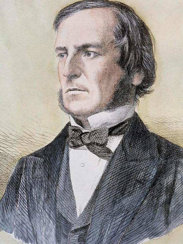
    George Boole (Wikipedia)

Agent, AI agent or an intelligent agent is used often to describe algorithms or AI systems that are released by research teams recently. However, the definition of an intelligent agent (IA) is a bit opaque. Naïvely thinking, it is nothing more than a decision maker that shows some intelligent behaviour. However, making a decision intelligently is hard to quantify computationally, and probably IA for us is something that can be representable as a Turing machine.  Here, we argue that an intelligent agent in the current AI systems should be seen as a function without side effects outputting a boolean output and shouldn't be extrapolated or compare to human level intelligence.  Causal inference capabilities should be seen as a scientific guidance to this function decompositions without side-effects,  i.e., Human in-the loop Probabilistic Boolean Functions (PBFs).

Computational learning theories are based on binary learners

Two of the major  theories of statistical learning PAC and VC dimensions build upon on "binary learning".  

PAC stands for Probably Approximately Correct, It sets basic framework and mathematical building blocks for defining a machine learning problem from complexity theory. Probably correct implies finding a weak learning function given binary instance set $X=\{1,0\}^{n}$. The binary set or its subsets mathematically called concepts and under certain mathematical conditions a system said to be PAC learnable. There are equivalences to VC and other computation learning frameworks. 

Robust AI systems: Deep reinforcement learning and  PAC

Even though the theory of learning on deep (reinforcement) learning is not established and active area of research. There is an intimate connection with composition of concepts, i.e., binary instance subsets as almost all operations within  deep RL can be viewed as probabilistic Boolean functions (PBFs). 

Conclusion 

Current research and practice in robust AI systems could focus on producing learnable probabilistic boolean functions (PBFs) as intelligent agents, rather than being a human level intelligent agents. This modest purpose might bring more practical fruit than long-term aims of replacing human intelligence. Moreover, theory of computation for deep learning and causality could benefit from this approach. 

Further reading

• Valiant84. Theory of Learnable.
• VC Dimension.
• Modern Theory and Machine Learning, Chase-Freitag, 2018